hands on machine learning

SKlearn

common符号

m is the number of instance
$x^{(i)}$a vector of all feature value of the $i^{th}$ instance
X is a matrix containing all feature values(excluding labels)
$$\left(\begin{array}{c}{\left(x^{(1)}\right)}^T\\ {\left(x^{(2)}\right)}^T\\ ...\\ {\left(x^{(2000)}\right)}^T\end{array}\right)$$
h is prediciton function, also called hypothesis
$\hat{y}=h(x^{(1)})=158,300$

ONneHotEncoder p67

p67
假设一个n行column有m个不同categorical 元素，那么会将其转换成n $\times$ m 的稀疏矩阵，对应 元素为1，其他元素为0.

Grid Search p76

Try all permutation of hyper parameters with a chosen estimator, return the best one.
代码如下

from sklearn.model_selection import GridSearchCV
param_grid = [
   {'n_estimators': [3,10,30], 'max_features': [2,4,6,8]}
   {'bootstrap': [False],  'n_estimators': [3, 10], 'max_features': [2,3,4]},
   ]
forest_reg = RandomForestRegressor()
grid_search = GridSearchCV(forest_reg, param_grid, cv=5,
   							scoring='neg_mean_squared_error',
   							return_train_score=True)
grid_search.fit(housing_prepared, housing_labels)

GridSearchCV.best_params_ 返回dict类型的params
GridSearchCV.best_estimator_ 返回最优estimator

For more randomness, try from sklearn.model_selection import RandomizedSearchCV on page #78.

如何测试结果 p79

1.pipeline.transform(X_test)
2. pipeline.transform(Y_test) //X，Y来自test_set
3. final_predictions = final_model.predict(X_test_prepared)
4. final_mse = mean_squared_error(y_test, final_predictions)
5. final_rmse = np.sqrt(final_mse)

SDGClassifier p88

Stochastic Gradient Descent （一个linear model）

from sklearn.linear_model import SDGClassifier
sgd_clf = SDGClassifier(random_state=42)
sgd_clf.fit(X_train, y_train)

• 计算loss function随意选择一个sample，而不是计算对于所有的loss的和。
• 比普通gradient更快

cross_va_predict p90

代码如下

from sklearn.model_selection import cross_val_predict
y_train_pred = cross_val_predict(<estimator>, X_train, y_train_5, cv = 3)
这里estimator不用被fit， 所有的prediction都是‘clean'的（没有被用到train set）

confusion_matrix p90

$\left(\begin{array}{cc}53057,& 1522\\ 1325,& 4096\end{array}\right)$ = $\left(\begin{array}{cc}TrueNegative(TN),& FalsePositive(FP)\\ FalseNegative(FN),& TruePositive(TP)\end{array}\right)$
$-------------------------------$
Precision = $\frac{TP}{TP+FP}$, 接近于1说明”留下的都是好人“

Recall = $\frac{TP}{TP+FN}$, 接近于1说明”好人都被留下了”

代码如下

from sklearn.metrics import confusion_matrix
confusion_matrix(actural, predicted)
#precision and recall
from sklearn.metrics import precision_score, recall_score
precision_score(y_train_5, y_train_pred)
recall_score(y_train_5, y_train_pred)

receiver operating characteristic (ROC) curve p97

plot true positive rate (recall) against false positive rate
True positive rate = recall = $\frac{TP}{TP+FP}$,

false positive rate (FPR) = $\frac{FP}{FP+TN}$,

from sklearn.metrics import roc_curve
fpr, tpr, thresholds = roc_curve(y_train_5, y_scores)
plt.plot(fpr, tpr, linewidth=2, label=label)

OvR, OvO p100

OvR: one-versus the rest

• run n 次，看哪个class得分最高

OvO: one-versus-one

• run $\frac{N\ast (N-1)}{2}$次，看那个类赢的duel次数最多

from sklearn.multiclass import OneVsRestClassifier #或者OneVsOneClassfier
ovr_clf = OneVsRestClassifier(SVC())
ovr_clf.fit(X_train, y_train)

Linear Regression

$\hat{y}={\theta }_0+{\theta }_1{x}_1+...+{\theta }_n{x}_n$
注意${\theta }_0$是bias， 再与x相乘的时候要 add x0 = 1 to each instance

X_b = np.c_[np.ones((100,1)), X]
Normal Equation:
theta_best = np.linalg.inv(X_b.T.dot(X_b)).dot(X_b.T).dot(y)

support vector machine

Binary classifier

如果结果不是binary， sklearn自动run OvO

from sklearn.svm import SVC
svm_clf = SVC()
svm_clf.fit(X_train, y_train)
svm_clf.predict([some_digit])
#或者SGD也可以

TF embedding layer

吧一个categorical data转换为(64) demensional vector. 越接近的category的vector角度之间越小

import tensorflow as tf
from tensorflow import keras
import numpy as np
model = keras.Sequential()
model.add(tf.keras.layers.Embedding(1000, 64, batch_input_shape=[32, None]))
y = model.predict([5])
y.shape
#(1,1,64)

softmax

$$softmax(x_i)=\frac{\exp (x^i)}{{\sum }_{j=1}^n\exp (x^j)}$$

PCA p225

project to low dimensional space, keeping the maximum variance

SVD: Singular Value Decomposition, 一个theorem that 任何matrix $A_{mn}$都可以转换成$U_{mm}{S}_{mn}{V}_{nn}^T$,

SVD详细介绍以及算法
V就是我们的principal ccomponent.
这里$U,V^T$是orthogonal matrix, aka $U^{T}U=I$, S 是diagonal matrix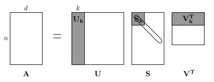

Incremental PCA (IPCA)

split the training set into mini-batches.

Kernel PCA (KPCA)

uses the kernel trick, RBF kernel for example.
use gridSearch to selsect the kernel and hyperparaeters.

LLE

Manifold learning technique
First measuring how each training instance linearly relates to its cloest neighbors
then looking for a low-dimentsional representation of the training set where theses local relationsips are best preserved.
$$\begin{gathered} \hat{W}=\underset{w}{\mathrm{argmin}}(x^{(i)}\sum _{j-1}^m{w}_{i,j}{x}^{(j)}) \\ \text{subject to}\{\begin{array}{ll}{w}_{i,j}=1& if{x}^{(j)}\text{is not one of the k c.n. of }x(i)\\ {\sum }_{j=1}^m{w}_{i,j}=1& fori=1,2,...,m\end{array} \end{gathered}$$
W是一个m x m的矩阵，W_i 的sum为1，$w_{i.j}$越大代表$x^{(i)},x^{(j)}$越接近
然后我们寻咋$\hat{z}$
$$\hat{Z}=\underset{Z}{\mathrm{argmin}}\sum _{i=1}^m(z^{(i)}-\sum _{j=1}^m{\hat{w}}_{i,j}{z}^{(j)}{)}^2$$
complexity: $O(m\log (m)n\log (k))$ for knn, $O(mn{k}^3)$ for optimizing the wieght, and $O(d{m}^2)$ for constructing z

K-Means p239

unsupervised learning,找到k个centroid
inertia是 mean squared distance betwee neach instance and its closest centroid.
k越大ineratia越小
怎么选k？plot inertia下降曲线，选转折点（coarse approach)
silhouette score

mean silhouette coefficient over all the instances.
silhouette coefficient is equal to (b-1) / max(a, b)
a is the mean distance to the other instances

from sklearn.cluster import KMeans
k = 5
kmeans = KMeans(N_cluster=k)
y_pred = kmeans.fit_predict(X)
>>> y_pred
>array([4,0,1, ... , 2, 1 0], dtype=int32
>>>kmeans.cluster_centers_
array([[-2.8, 1.8],
[0.2, 2.2], 
[-2.7, 2,7],
[-1.4, 2.2],
[-2.8, 1.3]])

Process

1. start by placing the centroids randomly
2. lavel the instances
3. update the centroids
4. repeat 2 and 3

we can avvoid unluckiness by

good_init = np.array([[-3,3],[-3,2], [-3,1], [-1,2], [0,2]])
kmeans = KMeans(n_clusters=5, init=good_init, n_init - 1)

Or trying more
or

K_Means++

1. Take one random centroid $c^{(1)}$
2. chosse an instand $x(i)$ with probability $D(x(i){)}^2/{\sum }_{j=1}^{m}D(x^{(j)}{)}^2$

Accelerated K-Means – by Charles Elkan
use triangle inequality

MiniBatchKMeans

as title, use mini batches
speeds up by three or four

Gaussian Mixtures

假设每个clusture都是高斯分布

If $z^{(i)}=j$,then $x^{(i)}\widetilde{.}N(u^{(j)},{\sigma }^{(j)}).$
其他类型Kmeans
BIRCH
处理大数据
Mean-Shift

Tensorflow

Perceptron

和neuron差不多（应该？） 每个perceptron有一个z， $z=w^{T}w$, 然后有一个threshold。
$$heaviside(z)=\{\begin{array}{ll}0& z<0\\ 1& z\ge 0\end{array}$$
每一层都会有bias，有额外的neuron来表示。这个neuron没有input edge只有output edge

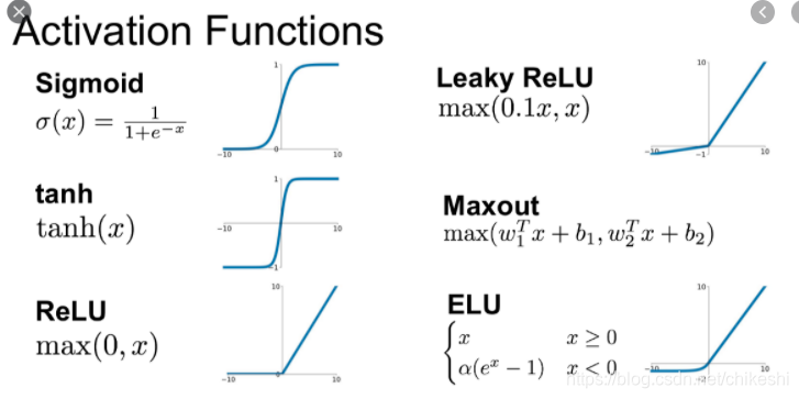
Activation functions p292

没有non linearity的话MLP(mult layer perceptions)就只是一个single layer

Leaky Relu

$$LReLU(x)=max(\alpha x,x)$$

Parametric leaky ReLU

$$PReLU(x)=max(\alpha x,x),\text{a is trainable}$$

Scaled ELU (SELU)

$$SELU(x)=\lambda \{\begin{array}{ll}x& x\ge 0\\ a(e^x-1)& x<0\end{array}$$
比ELU多了个lambda， 貌似是最好用的

Complex Models

Wide & Deep nn p309

吧input层和最后的hidden layer直接拼在一起然后通过output layer

• 可以使模型capture最基础的特征

Keras多种用法

Subclassing API to build dynamic models p313

keras.Model可以被继承

Save a model p314

Using Callbacks p315

在model.fit里加上 callbacks=[f1,f2...], 这里f1,f2是keras.callbacks里的方法

TensorBoard p317

一个interactive visualization tool to view the leanrning curves during tranning.

Grid Search p321

RandomizedSearchCV(keras_reg, param_distribs, n_iter=10, cv=3)

zooming

when a region of parameter space is good, search more in it``

Vanishing/Exploding Gradient problem p332

Q； 不太懂为什么会梯度消失，既然每neuron都是下一层的总和

• 下一层有正有负，所以当做每层只有一个neuron就好

Xavier/Glorot initialization

fan_in: the number of inputs of a layer
fan_out: the number neurons of a layer
fan_avg = (fan_in + fan_out)/2

两种方式：normal distribution with mean 0 and variance $\sigma =\frac{1}{fa{n}_{avg}}$
或者 uniform idstribution between -r and +r, with $r=\sqrt{\frac{3}{fa{n}_{avg}}}$

Initialization	Activation functions	variance
Glorot	None, tanh, logistic, softmax	1/fan_avg
He	ReLU and variants	2/fan_in
LeCun	SELU	1/fan_in

Mean是0非常重要，否则有可能explode

Nonsaturating Activation Functions:

Nonsaturating activation function指的是𝑓 is non-saturating iff (|lim𝑧→−∞𝑓(𝑧)|=+∞)∨(|lim𝑧→+∞𝑓(𝑧)|=+∞)
saturating 有左右边界

Batch Normalization

let the model learn the optimal scale and mean of eacho f the layer’s inputs
B指的是mini-batch B
$$\begin{gathered} u_B=\frac{1}{m_B}\sum _{i=1}^B{x}^{(i)} \\ {\sigma }_B^2=\frac{1}{m_B}\sum _{i=1}^B(x^{(i)}-u_B{)}^2 \\ {\hat{x}}^{(i)}=\frac{x-u_B}{\sqrt{{\sigma }_B^2+ϵ}} \\ {\hat{z}}^{(i)}=\gamma \otimes x^{(i)}+\beta \end{gathered}$$
$\gamma ,\beta$ 是我们要训练的
train的时间增加，但runtime的速度一样，因为原本的$XW+b\to \gamma \otimes (XW+b)+\beta$

Gradient Clipping

如果gradient 大于1 / 小于 -1， 那么限制他在[1,-1]之内

Transfer Learning p348

reuse pretrained layer
迁移学习在low level feature相似的情况下效果最好
lower layer 对应 low level feature
upper layer 对应 upper level feature
所以我们要去掉深的层，留下浅的并把它锁住。
lower level feature例子： first order image gradients

Pretraining on an Auxiliary Task

如果transfer learning没有类似model怎么办？

• 自己训练一个
  比如我想训练识别猫头鹰，但没有很多照片
  如果我有很多鸟类照片，可以先训练个识别鸟类的model
  锁住model，加上几层继续训练

Optimizer

Momentum Optimizer

$$\begin{gathered} m\leftarrow {\beta }_{1}m-\eta {\nabla }_{\theta }J(\theta ) \\ \theta \leftarrow \theta -m \end{gathered}$$

Nesterov Accelerated Gradient

$$\begin{gathered} m\leftarrow \beta m-\eta {\nabla }_{\theta }J(\theta +\beta m) \\ \theta \leftarrow \theta +m（\eta =0.001,\beta =0.9\text{ by default}) \end{gathered}$$
吧正常的 $\theta$ 变成了 $\theta +\beta m$, 计算了稍稍往前一点地方的gradient

AdaGrad

scale down the gradient vector along the steepest dimensions.
减少梯度高的梯度，为了更好的朝中心下降。
会让training变慢，但下的比较快
$$\begin{gathered} s\leftarrow s+{\nabla }_{\theta }J(\theta )\otimes {\nabla }_{\theta }J(\theta ) \\ \theta \leftarrow \theta -\eta {\nabla }_{\theta }J(\theta )\oslash \sqrt{s+ϵ} \end{gathered}$$
不要用在DNN里，会过早停下训练。（在最低点周围的gradient很小，square一下几乎就没有了）

RMSProp

$$\begin{gathered} s\leftarrow \beta s+(1-\beta ){\nabla }_{\theta }J(\theta )\otimes {\nabla }_{\theta }J(\theta ) \\ \theta \leftarrow \theta -\eta {\nabla }_{\theta }J(\theta )\oslash \sqrt{s+ϵ} \end{gathered}$$

这会让s小一点，于是$\theta$就大一点 芜湖~

Adam and Nadam

芜湖，最常见的出现了
$$ m \leftarrow \beta_2 m - \eta \nabla_\theta J(\theta)\
s \leftarrow \beta_1 s +(1-\beta_1) \nabla_\theta J(\theta) \otimes \nabla_\theta J(\theta) \
\hat m \leftarrow \frac{m}{1-a^n}\

\theta \leftarrow \theta - m\
\theta \leftarrow \theta - \eta \nabla_\theta J(\theta) \oslash \sqrt{s+\epsilon}
$$

RNN(LSTM)

sigmoid表示gate，0-1的probalility

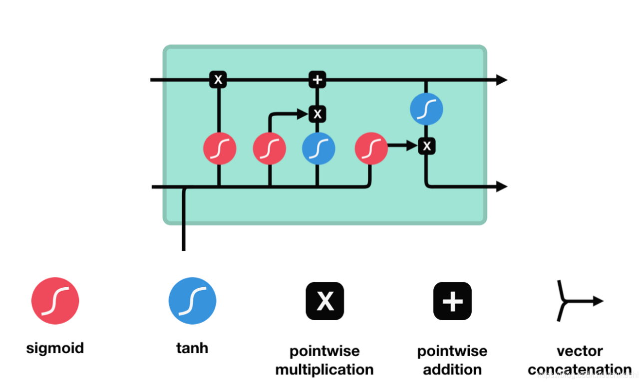
从左往右，第一个sigmoid, $f_t$表示forget gate ：$$f_t=\sigma (W_f{x}_t+U_f{h}_{t-1}+b_f)$$

• Wf: input weight for the forget gate
• Uf: recurrent weight for the forget gate
• bf: bias weight for the forget gate

从左往右，第二个sigmoid， $i_t$ 表示 update gate: $$i_t=\sigma (W_i{x}_t+U_i{h}_{t-1}+b_i)$$

• Wi: input weight for the update gate
• Ui: recurrent weight for the update gate
• bi: bias weight for the update gate.

从左往右，第一个tanh, $\widetilde{c_t}$ 表示 update candidate value.(注意这里是${\sigma }_h)$ $$\widetilde{c_t}={\sigma }_h(W_c{x}_T+U_c{h}_{t-1}+b_c)$$

• Wc: input weight for the candidate value
• Uc: recurrent weight for the candidate value
• bi: bias weight for the candidate value

新的state $C_t$: $$C_t=f_t\ast C_{t-1}+i_t\ast {\tilde{C}}_t$$
注意这里左右两个乘号分别对应图中两个乘号，加号对应图中的加号

从左往右，第三个sigmoid, $o_t$ 表示 output gate. $$o_t={\sigma }_g(W_o{x}_t+U_o{h}_{t-1}+b_o)$$

• Wo: input weight for the output gate
• Uo: recurrent weight for the output gate
• bo: bias weight for the output gate

从左往右，第二个tanh 表示final output
$$h_t=o_t\ast tanh(C_t)$$

$W_f$: input weight for the forget gate
$U_f$: recurrent weight for the forget gate
$b_f$: bias weight for the forget gate
$W_i$: input weight for the update gate
$U_i$: recurrent weight for the update gate
$b_i$: bias weight for the update gate.
$W_c$: input weight for the candidate value
$U_c$: recurrent weight for the candidate value
$b_i$: bias weight for the candidate value
$W_o$: input weight for the output gate
$U_o$: recurrent weight for the output gate
$b_o$: bias weight for the output gate
So there you have it, there are 12 weights that can largely be divided into three camps:
input weight that multiplies with the input timestep
recurrent weight that multiplies with the previous output
bias weight

Q&A

• tanh 的值是是[-1,1], $o_t$的值是[0,1], 那最后$h_t$的output不就是[0,1]?
• sigmoid是处理forget的概率，tanh是处理值
• 这里貌似并没有DNN，只有matrix multiplicaiton。一个matmul代表不了DNN因为没有non-linarity

code level of LTSM

原文地址
pre-knowledge: Keras Layer class
Three important functions: __init()__, __build()__ , __call()__
可以在init里面设置weight(w)和bias(b), 推荐在build里面
init会在被创建的时候运行，build会在第一次run的时候运行

def build(self, input_shape):
	input_dim = input_shape[-1]
	...
	self.kernel = self.add_weight(shape=(input_dim, self.units * 4), ...)

这里4*self.units是因为i(update) f(forget) c(update candidate) o(output)各需要一个

def call(self, inputs, states, training=None):
	...
	 h_tm1 = states[0]  # previous memory state
     c_tm1 = states[1]  # previous carry state
	i = self.recurrent_activation(x_i + K.dot(h_tm1_i,
	                                       self.recurrent_kernel_i))
	f = self.recurrent_activation(x_f + K.dot(h_tm1_f,
	                                       self.recurrent_kernel_f))
	c = f * c_tm1 + i * self.activation(x_c + K.dot(h_tm1_c,
	                                             self.recurrent_kernel_c))
	o = self.recurrent_activation(x_o + K.dot(h_tm1_o,
	                                       self.recurrent_kernel_o)
	...
	h = o * self.activation(c)

这几行分别对应上面几个式子。
注意self.recurrent_activation和self_activation是不同的。一般recurrent_activation是Sigmoid，activation是tanh，不过可以自己设定

GRU

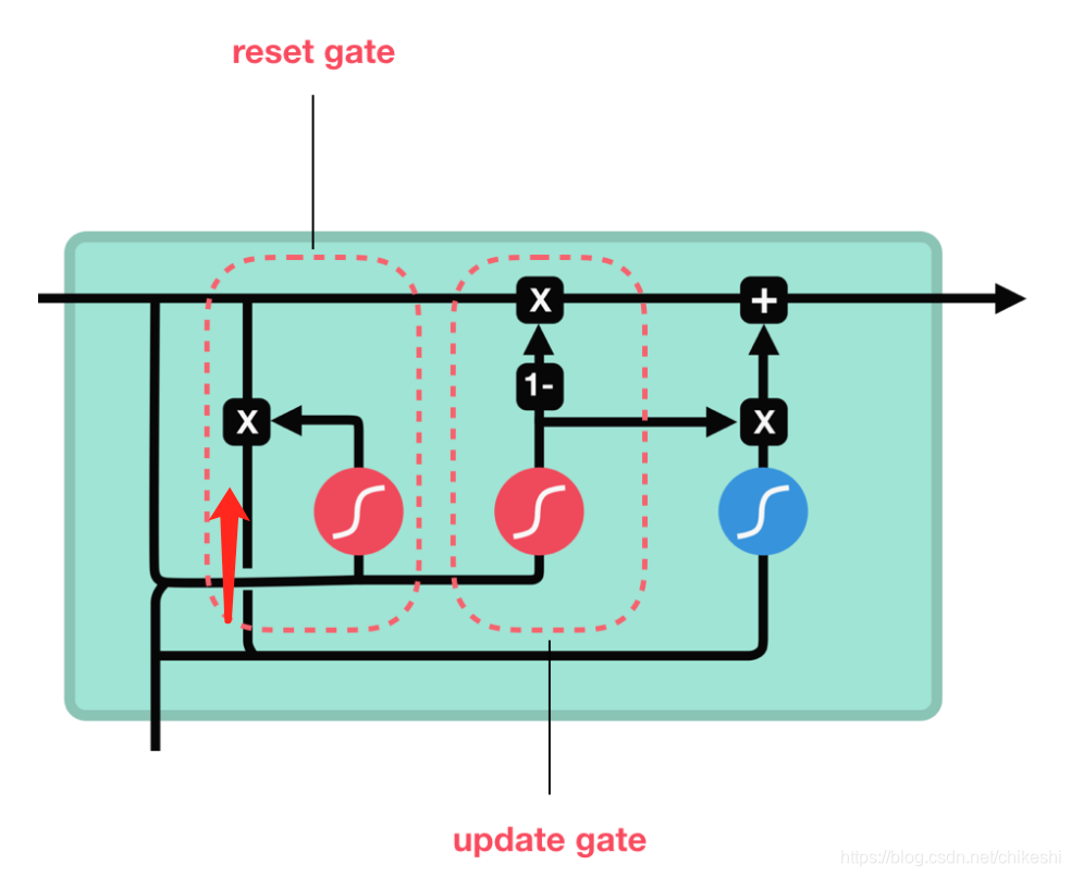
Update gate:
$$U_t=\sigma (W_u{h}_{t-1}+U_u{x}_t{b}_u)$$
Reset gate:
$$r_t=\sigma (W_r{h}_{t-1}+U_t{x}_t+b_r)$$
New hidden state content:
$${\tilde{h}}_t=\tanh (W_h(r_t\otimes h_{t-1}+U_h{x}_t+b_h)$$
Hidden State:
$$h_t=(1-u_t)\otimes h_{t-1}+u_t\otimes {\tilde{h}}_t$$