从零开始逐步指导开发者构建自己的大型语言模型（LLM）学习笔记- 第3章编码注意力机制Coding Attention Mechanisms_serrano.academy attention mechanisms in llms-优快云博客

本文链接：https://blog.youkuaiyun.com/chenchihwen/article/details/144936755

这段文本主要介绍了 “Chapter 3: Coding Attention Mechanisms”（第三章：编码注意力机制）的相关资料。

其中，“Main Chapter Code”（主章节代码）部分，

代码存于 [01_main-chapter-code] 中；

“Bonus Materials”（额外资料）部分包含两方面内容，

一是 [02_bonus_efficient-multihead-attention] 实现并比较了多头注意力的不同实现变体，

二是 [03_understanding-buffers] 阐释了 PyTorch 缓冲区背后的概念，该缓冲区在第三章用于实现因果注意力机制。

Chapter 3: Coding Attention Mechanisms

《从头构建大语言模型》（Build a Large Language Model From Scratch）一书中关于注意力机制编码的章节，围绕注意力机制这一 LLMs 的核心引擎展开，详细介绍了多种注意力机制的原理、代码实现及应用，具体内容如下：

Packages that are being used in this notebook:

[1]

from importlib.metadata import version

print("torch version:", version("torch"))
torch version: 2.4.0

This chapter covers attention mechanisms, the engine of LLMs:

3.1 The problem with modeling long sequences

长序列建模难题：在机器翻译任务中，逐词翻译因源语言和目标语言的语法结构差异而不可行。在 Transformer 模型出现之前，编码器 - 解码器 RNNs 常用于机器翻译，编码器通过隐藏状态生成输入序列的浓缩表示。
注意力机制的作用：通过注意力机制，网络的文本生成解码器部分能够有选择地访问所有输入令牌，意味着某些输入令牌在生成特定输出令牌时更重要。自注意力是一种增强输入表示的技术，使序列中的每个位置能够与其他位置相互作用并确定相关性。
Translating a text word by word isn't feasible due to the differences in grammatical structures between the source and target languages:

Prior to the introduction of transformer models, encoder-decoder RNNs were commonly used for machine translation tasks
In this setup, the encoder processes a sequence of tokens from the source language, using a hidden state—a kind of intermediate layer within the neural network—to generate a condensed representation of the entire input sequence:

- 在引入变压器模型之前，编码器 - 解码器循环神经网络（RNN）通常用于机器翻译任务。
- “变压器模型”指的是一种特定的机器学习模型，通常在自然语言处理等领域有广泛应用。
- “编码器 - 解码器循环神经网络（RNN）”是一种用于处理序列数据的神经网络结构，由编码器和解码器两部分组成，在机器翻译中，编码器将源语言的序列转换为一种中间表示，解码器再将这种中间表示转换为目标语言的序列。
- “机器翻译任务”即把一种语言的文本自动转换为另一种语言的文本的任务。
- 在这种设置中，编码器处理来自源语言的一系列标记，使用隐藏状态（神经网络中的一种中间层）来生成整个输入序列的浓缩表示。
- “设置”在这里指的是使用编码器 - 解码器 RNN 进行机器翻译的这种情况。
- “源语言”是要进行翻译的原始语言。
- “一系列标记”可以理解为源语言文本被分割成的一个个单元，比如单词或字符等。
- “隐藏状态”是 RNN 中的一种内部状态，它在处理序列数据的过程中不断更新，用于存储对之前输入的信息的记忆，从而帮助网络更好地理解当前的输入和生成输出。
- “中间层”是神经网络中的一层，在编码器 - 解码器 RNN 中，隐藏状态所在的层起到了连接输入和输出的中间作用，它将输入序列进行编码，生成一个能够代表整个序列的浓缩表示。
- “浓缩表示”是对输入序列的一种简化和抽象，它包含了输入序列的关键信息，以便解码器能够根据这个表示来生成目标语言的输出。
- “整个输入序列”即源语言的文本序列。

3.2 Capturing data dependencies with attention mechanisms

章节 3.2， “利用注意力机制捕获数据依赖关系”。这里可能是在讨论一种技术方法，即通过注意力机制来获取数据之间的依赖关系，注意力机制通常用于有选择地关注输入数据的特定部分，从而更好地理解数据的结构和关系。在特定的技术领域，如机器学习、深度学习等领域，这可能涉及到对数据特征的提取和分析，以提高模型的性能和准确性。

No code in this section
Through an attention mechanism, the text-generating decoder segment of the network is capable of selectively accessing all input tokens, implying that certain input tokens hold more significance than others in the generation of a specific output token:

通过注意力机制，网络的文本生成解码器部分能够有选择地访问所有输入标记，这意味着在生成特定输出标记时，某些输入标记比其他标记更重要。

Self-attention in transformers is a technique designed to enhance input representations by enabling each position in a sequence to engage with and determine the relevance of every other position within the same sequence

在 Transformer 中，自注意力（Self-attention）是一种旨在通过使序列中的每个位置都能够与同一序列中的其他每个位置进行交互并确定其相关性，从而增强输入表示的技术。

具体来说，自注意力机制允许模型在处理一个序列时，不同位置的元素能够根据彼此的重要性进行动态调整权重。例如在自然语言处理任务中，一个句子中的不同单词可以通过自注意力机制来确定彼此对于当前任务的重要程度。这样可以更好地捕捉句子中的长距离依赖关系以及不同部分之间的复杂语义联系。

比如在翻译任务中，模型可以利用自注意力机制来确定源语言句子中哪些单词对于目标语言的翻译结果最为关键，从而更准确地进行翻译。同时，自注意力机制也使得模型能够并行地处理整个序列，提高了计算效率。

3.3 Attending to different parts of the input with self-attention

3.3 使用自注意力关注输入的不同部分

3.3.1 A simple self-attention mechanism without trainable weights一种没有可训练权重的简单自注意力机制）

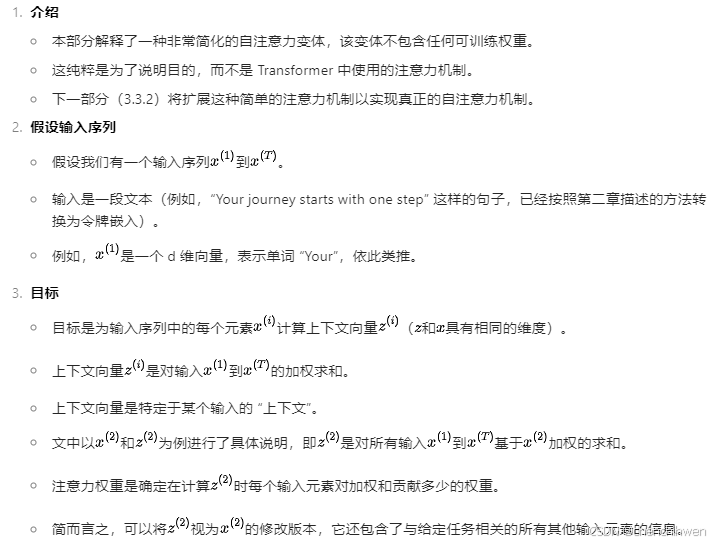
This section explains a very simplified variant of self-attention, which does not contain any trainable weights
This is purely for illustration purposes and NOT the attention mechanism that is used in transformers
The next section, section 3.3.2, will extend this simple attention mechanism to implement the real self-attention mechanism
Suppose we are given an input sequence 𝑥(1)x(1) to 𝑥(𝑇)x(T)
- The input is a text (for example, a sentence like "Your journey starts with one step") that has already been converted into token embeddings as described in chapter 2
- For instance, 𝑥(1)x(1) is a d-dimensional vector representing the word "Your", and so forth
Goal: compute context vectors 𝑧(𝑖)z(i) for each input sequence element 𝑥(𝑖)x(i) in 𝑥(1)x(1) to 𝑥(𝑇)x(T) (where 𝑧z and 𝑥x have the same dimension)
- A context vector 𝑧(𝑖)z(i) is a weighted sum over the inputs 𝑥(1)x(1) to 𝑥(𝑇)x(T)
- The context vector is "context"-specific to a certain input
  - Instead of 𝑥(𝑖)x(i) as a placeholder for an arbitrary input token, let's consider the second input, 𝑥(2)x(2)
  - And to continue with a concrete example, instead of the placeholder 𝑧(𝑖)z(i), we consider the second output context vector, 𝑧(2)z(2)
  - The second context vector, 𝑧(2)z(2), is a weighted sum over all inputs 𝑥(1)x(1) to 𝑥(𝑇)x(T) weighted with respect to the second input element, 𝑥(2)x(2)
  - The attention weights are the weights that determine how much each of the input elements contributes to the weighted sum when computing 𝑧(2)z(2)
  - In short, think of 𝑧(2)z(2) as a modified version of 𝑥(2)x(2) that also incorporates information about all other input elements that are relevant to a given task at hand

(Please note that the numbers in this figure are truncated to one
digit after the decimal point to reduce visual clutter; similarly, other figures may also contain truncated values)

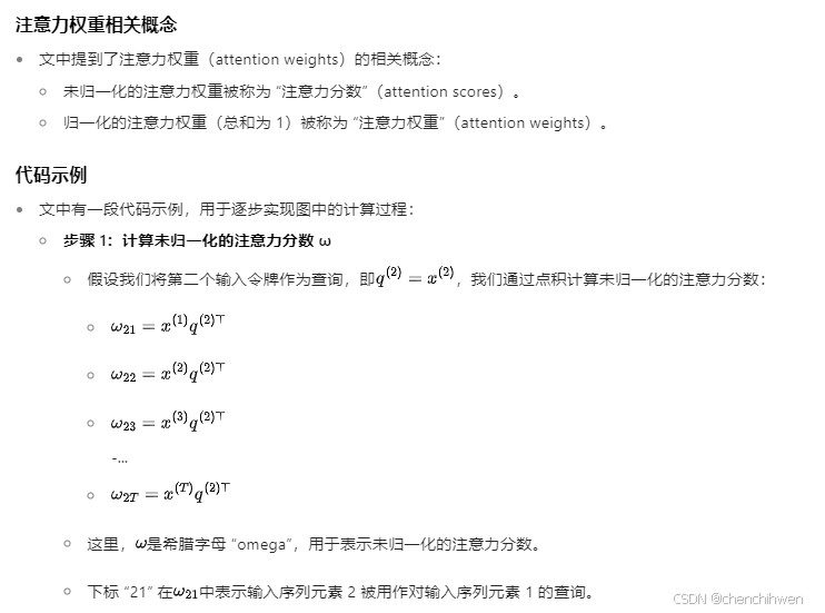
By convention, the unnormalized attention weights are referred to as "attention scores" whereas the normalized attention scores, which sum to 1, are referred to as "attention weights"

The code below walks through the figure above step by step

Step 1: compute unnormalized attention scores 𝜔ω
Suppose we use the second input token as the query, that is, 𝑞(2)=𝑥(2)q(2)=x(2), we compute the unnormalized attention scores via dot products:
- 𝜔21=𝑥(1)𝑞(2)⊤ω21=x(1)q(2)⊤
- 𝜔22=𝑥(2)𝑞(2)⊤ω22=x(2)q(2)⊤
- 𝜔23=𝑥(3)𝑞(2)⊤ω23=x(3)q(2)⊤
- ...
- 𝜔2𝑇=𝑥(𝑇)𝑞(2)⊤ω2T=x(T)q(2)⊤
Above, 𝜔ω is the Greek letter "omega" used to symbolize the unnormalized attention scores
- The subscript "21" in 𝜔21ω21 means that input sequence element 2 was used as a query against input sequence element 1

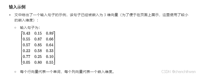
Suppose we have the following input sentence that is already embedded in 3-dimensional vectors as described in chapter 3 (we use a very small embedding dimension here for illustration purposes, so that it fits onto the page without line breaks):

[2]

import torch

inputs = torch.tensor(

[[0.43, 0.15, 0.89], # Your (x^1)

[0.55, 0.87, 0.66], # journey (x^2)

[0.57, 0.85, 0.64], # starts (x^3)

[0.22, 0.58, 0.33], # with (x^4)

[0.77, 0.25, 0.10], # one (x^5)

[0.05, 0.80, 0.55]] # step (x^6)

)

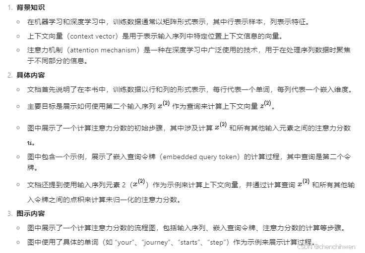
(In this book, we follow the common machine learning and deep learning convention where training examples are represented as rows and feature values as columns; in the case of the tensor shown above, each row represents a word, and each column represents an embedding dimension)
The primary objective of this section is to demonstrate how the context vector 𝑧(2)z(2)
is calculated using the second input sequence, 𝑥(2)x(2), as a query
The figure depicts the initial step in this process, which involves calculating the attention scores ω between 𝑥(2)x(2)
and all other input elements through a dot product operation

We use input sequence element 2, 𝑥(2)x(2), as an example to compute context vector 𝑧(2)z(2); later in this section, we will generalize this to compute all context vectors.
The first step is to compute the unnormalized attention scores by computing the dot product between the query 𝑥(2)x(2) and all other input tokens:

[3]

query = inputs[1] # 2nd input token is the query

attn_scores_2 = torch.empty(inputs.shape[0])

for i, x_i in enumerate(inputs):

attn_scores_2[i] = torch.dot(x_i, query) # dot product (transpose not necessary here since they are 1-dim vectors)

print(attn_scores_2)

tensor([0.9544, 1.4950, 1.4754, 0.8434, 0.7070, 1.0865])

Side note: a dot product is essentially a shorthand for multiplying two vectors elements-wise and summing the resulting products:

Step 2: normalize the unnormalized attention scores ("omegas", 𝜔ω) so that they sum up to 1
Here is a simple way to normalize the unnormalized attention scores to sum up to 1 (a convention, useful for interpretation, and important for training stability):

[5]

attn_weights_2_tmp = attn_scores_2 / attn_scores_2.sum()

print("Attention weights:", attn_weights_2_tmp)

print("Sum:", attn_weights_2_tmp.sum())

Attention weights: tensor([0.1455, 0.2278, 0.2249, 0.1285, 0.1077, 0.1656])

Sum: tensor(1.0000)

However, in practice, using the softmax function for normalization, which is better at handling extreme values and has more desirable gradient properties during training, is common and recommended.
Here's a naive implementation of a softmax function for scaling, which also normalizes the vector elements such that they sum up to 1:

[6]

def softmax_naive(x):

return torch.exp(x) / torch.exp(x).sum(dim=0)

attn_weights_2_naive = softmax_naive(attn_scores_2)

print("Attention weights:", attn_weights_2_naive)

print("Sum:", attn_weights_2_naive.sum())

Attention weights: tensor([0.1385, 0.2379, 0.2333, 0.1240, 0.1082, 0.1581])

Sum: tensor(1.)

The naive implementation above can suffer from numerical instability issues for large or small input values due to overflow and underflow issues
Hence, in practice, it's recommended to use the PyTorch implementation of softmax instead, which has been highly optimized for performance:

[7]

attn_weights_2 = torch.softmax(attn_scores_2, dim=0)

print("Attention weights:", attn_weights_2)

print("Sum:", attn_weights_2.sum())

Attention weights: tensor([0.1385, 0.2379, 0.2333, 0.1240, 0.1082, 0.1581])

Sum: tensor(1.)

Step 3: compute the context vector 𝑧(2)z(2) by multiplying the embedded input tokens, 𝑥(𝑖)x(i) with the attention weights and sum the resulting vectors:

[8]

query = inputs[1] # 2nd input token is the query

context_vec_2 = torch.zeros(query.shape)

for i,x_i in enumerate(inputs):

context_vec_2 += attn_weights_2[i]*x_i

print(context_vec_2)

tensor([0.4419, 0.6515, 0.5683])

3.3.2 Computing attention weights for all input tokens

Generalize to all input sequence tokens:

Above, we computed the attention weights and context vector for input 2 (as illustrated in the highlighted row in the figure below)
Next, we are generalizing this computation to compute all attention weights and context vectors

接下来的步骤是将上述计算推广到所有输入序列的标记，即计算每个标记的注意力权重和上下文向量。这段代码的目的是为了说明如何将注意力机制的计算从单个标记扩展到整个输入序列，以便更好地理解和处理序列数据。

(Please note that the numbers in this figure are truncated to two
digits after the decimal point to reduce visual clutter; the values in each row should add up to 1.0 or 100%; similarly, digits in other figures are truncated)

In self-attention, the process starts with the calculation of attention scores, which are subsequently normalized to derive attention weights that total 1
These attention weights are then utilized to generate the context vectors through a weighted summation of the inputs

Apply previous step 1 to all pairwise elements to compute the unnormalized attention score matrix:

Apply previous step 3 to compute all context vectors:

[13]

3.4 Implementing self-attention with trainable weights

A conceptual framework illustrating how the self-attention mechanism developed in this section integrates into the overall narrative and structure of this book and chapter

3.4.1 Computing the attention weights step by step

自注意力机制（self-attention mechanism），也被称为 “缩放点积注意力”（scaled dot-product attention）。以下是详细解释：

整体内容概述

这段文本主要讲解了在原始 Transformer 架构、GPT 模型以及大多数其他流行的大型语言模型（LLMs）中使用的自注意力机制的实现步骤。它提到了计算注意力权重的总体思路，并指出与之前介绍的基本注意力机制相比，主要的不同在于引入了在模型训练过程中更新的权重矩阵，这些可训练的权重矩阵对于模型（特别是模型内部的注意力模块）能够学习生成 “良好” 的上下文向量至关重要。

具体内容解析

自注意力机制的应用范围：
- 文中明确指出，在这一部分，正在实现的自注意力机制被用于原始 Transformer 架构、GPT 模型以及大多数其他流行的大型语言模型中。这表明自注意力机制是这些先进模型的核心组成部分，对于它们的性能和功能起着关键作用。
自注意力机制的名称：
- 这种自注意力机制也被称为 “scaled dot-product attention”，即缩放点积注意力。这是该机制在技术领域的常见术语，了解这个名称有助于在相关技术交流和研究中准确识别和理解。
总体思路：
- 总体思路与之前类似，主要包括两个方面：
  - 想要计算特定输入元素的上下文向量，这些上下文向量是输入向量的加权和。这意味着模型需要根据输入元素的不同，为每个输入向量分配不同的权重，然后通过加权求和来得到上下文向量，从而更好地理解输入的语义和上下文信息。
  - 为了实现上述计算，需要注意力权重。注意力权重决定了每个输入向量在计算上下文向量时的重要性程度，是自注意力机制的核心要素之一。
与基本注意力机制的差异：
- 与之前介绍的基本注意力机制相比，最显著的差异是引入了在模型训练过程中更新的权重矩阵。这些权重矩阵是可训练的，通过在大量数据上进行训练，模型能够学习到合适的权重值，使得注意力模块能够生成更 “好” 的上下文向量。这里的 “好” 可以理解为更能准确反映输入元素之间的语义关系和上下文信息，从而提高模型在各种自然语言处理任务中的性能，如语言理解、生成、翻译等。

In this section, we are implementing the self-attention mechanism that is used in the original transformer architecture, the GPT models, and most other popular LLMs
This self-attention mechanism is also called "scaled dot-product attention"
The overall idea is similar to before:
- We want to compute context vectors as weighted sums over the input vectors specific to a certain input element
- For the above, we need attention weights
As you will see, there are only slight differences compared to the basic attention mechanism introduced earlier:
- The most notable difference is the introduction of weight matrices that are updated during model training
- These trainable weight matrices are crucial so that the model (specifically, the attention module inside the model) can learn to produce "good" context vectors

Implementing the self-attention mechanism step by step, we will start by introducing the three training weight matrices 𝑊𝑞Wq, 𝑊𝑘Wk, and 𝑊𝑣Wv
These three matrices are used to project the embedded input tokens, 𝑥(𝑖)x(i), into query, key, and value vectors via matrix multiplication:
- Query vector: 𝑞(𝑖)=𝑊𝑞𝑥(𝑖)q(i)=Wqx(i)
- Key vector: 𝑘(𝑖)=𝑊𝑘𝑥(𝑖)k(i)=Wkx(i)
- Value vector: 𝑣(𝑖)=𝑊𝑣𝑥(𝑖)v(i)=Wvx(i)

The embedding dimensions of the input 𝑥x and the query vector 𝑞q can be the same or different, depending on the model's design and specific implementation
In GPT models, the input and output dimensions are usually the same, but for illustration purposes, to better follow the computation, we choose different input and output dimensions here:

[15]

初始化 W QKV

计算

In the next step, step 2, we compute the unnormalized attention scores by computing the dot product between the query and each key vector:

[19]

Since we have 6 inputs, we have 6 attention scores for the given query vector:

[20]

attn_scores_2 = query_2 @ keys.T # All attention scores for given query

print(attn_scores_2)

tensor([1.2705, 1.8524, 1.8111, 1.0795, 0.5577, 1.5440])

Next, in step 3, we compute the attention weights (normalized attention scores that sum up to 1) using the softmax function we used earlier
The difference to earlier is that we now scale the attention scores by dividing them by the square root of the embedding dimension, 𝑑𝑘⎯⎯⎯⎯√dk (i.e., d_k**0.5):

[21]

In step 4, we now compute the context vector for input query vector 2:

3.4.2 Implementing a compact SelfAttention class

Putting it all together, we can implement the self-attention mechanism as follows:

Python类的构造函数，用于初始化一个自注意力机制（Self-Attention）的模型。具体来说，这个类是 SelfAttention_v1，它继承自 nn.Module，这是PyTorch中用于定义神经网络模块的基类。构造函数 __init__ 接受两个参数：d_in 和 d_out，分别表示输入特征的维度和输出特征的维度。在构造函数内部，首先调用了父类的构造函数 super().__init__()，以确保父类的初始化过程被正确执行。然后，构造函数定义了三个可学习的参数：W_query、W_key 和 W_value，它们都是 nn.Parameter 类型的张量。这些参数在模型训练过程中会被自动优化。每个参数都是通过 torch.rand 函数随机初始化的，其形状为 (d_in, d_out)，即输入特征的维度乘以输出特征的维度。这些参数在自注意力机制中扮演着重要的角色： • W_query：用于将输入特征映射到查询空间。 • W_key：用于将输入特征映射到键空间。 • W_value：用于将输入特征映射到值空间。在自注意力机制中，查询（query）、键（key）和值（value）是通过这些参数与输入特征的矩阵乘法得到的。这些参数的初始化对于模型的性能和收敛速度有着重要的影响。

SelfAttention_v1 类的 forward 方法，它实现了自注意力机制的前向传播过程。以下是对这段代码的详细解释：

1. 计算键（keys）、查询（queries）和值（values）：

keys = x @ self.W_key
queries = x @ self.W_query
values = x @ self.W_value
这里，x 是输入张量，self.W_key、self.W_query 和 self.W_value 是在类的构造函数中定义的可学习参数。通过矩阵乘法，将输入 x 分别与这些参数相乘，得到键、查询和值。

2. 计算注意力分数（attention scores）：

attn_scores = queries @ keys.T
注意力分数是通过查询和键的转置之间的矩阵乘法计算得到的。这里的 @ 表示矩阵乘法，keys.T 表示键的转置。注意力分数衡量了查询和键之间的相关性。

3. 计算注意力权重（attention weights）：

attn_weights = torch.softmax(attn_scores / keys.shape[-1]**0.5, dim=-1)
注意力权重是通过对注意力分数应用 softmax 函数得到的。在计算 softmax 之前，注意力分数先除以键的维度的平方根（keys.shape[-1]**0.5），这是为了防止在计算 softmax 时出现数值上的不稳定。dim=-1 表示在最后一个维度上进行 softmax 操作。

4. 计算上下文向量（context vector）：

context_vec = attn_weights @ values
上下文向量是通过注意力权重和值之间的矩阵乘法计算得到的。注意力权重决定了每个值在上下文中的重要性，最终的上下文向量是这些值的加权和。

5. 返回上下文向量：

return context_vec
最后，forward 方法返回计算得到的上下文向量。这段代码实现了自注意力机制的核心计算过程，通过计算键、查询和值之间的相关性，得到注意力权重，然后利用这些权重对值进行加权求和，得到最终的上下文向量。这个上下文向量包含了输入序列中每个位置的信息，并且根据它们与当前位置的相关性进行了加权。

We can streamline the implementation above using PyTorch's Linear layers, which are equivalent to a matrix multiplication if we disable the bias units
Another big advantage of using nn.Linear over our manual nn.Parameter(torch.rand(...) approach is that nn.Linear has a preferred weight initialization scheme, which leads to more stable model training

**一、关于PyTorch的Linear层等同于无偏置单元的矩阵乘法**
1. 在神经网络中，线性层（nn.Linear）主要操作是进行线性变换。
- 当没有偏置单元（bias units）时，它的计算本质就是输入向量与权重矩阵相乘，这和手动定义参数进行矩阵乘法类似但更便捷高效。
**二、nn.Linear相对于手动nn.Parameter的优势**
1. 权重初始化方案
- nn.Linear有默认且推荐的权重初始化方式。
- 合适的初始化能让模型在训练初期就有较好的状态。例如，随机初始化权重如果不合适，可能导致梯度消失或爆炸等问题，而nn.Linear的初始化方案有助于避免这些问题，从而使模型训练过程更稳定，收敛更快。

Note that SelfAttention_v1 and SelfAttention_v2 give different outputs because they use different initial weights for the weight matrices

3.5 Hiding future words with causal attention

In causal attention, the attention weights above the diagonal are masked, ensuring that for any given input, the LLM is unable to utilize future tokens while calculating the context vectors with the attention weight
在因果注意力（causal attention）中，对角线以上的注意力权重被屏蔽。这意味着对于特定的输入，大型语言模型（LLM）在计算上下文向量与注意力权重时不能利用未来的标记（tokens）。比如说，在处理文本序列时，如果当前要处理第n个词，那么只能基于它之前（第1到n - 1个）的词的信息来确定注意力权重，而不能用到后面的词。这样做是为了符合逻辑顺序，因为在实际的语言理解和生成过程中，未来的信息是不可预知的。如果不进行这样的屏蔽，模型就会“作弊”，提前获取到后面的信息，从而不能准确地学习到基于当前及之前信息的合理表示，影响模型的泛化能力和生成内容的合理性。

3.5.1 Applying a causal attention mask

In this section, we are converting the previous self-attention mechanism into a causal self-attention mechanism
Causal self-attention ensures that the model's prediction for a certain position in a sequence is only dependent on the known outputs at previous positions, not on future positions
In simpler words, this ensures that each next word prediction should only depend on the preceding words
To achieve this, for each given token, we mask out the future tokens (the ones that come after the current token in the input text):

在这个部分，我们将把之前的自注意力机制转换为因果自注意力机制。因果自注意力确保模型对序列中某个位置的预测仅依赖于先前位置的已知输出，而不依赖于未来位置。简单来说，这确保了每个下一个单词的预测只应依赖于前面的单词。为了实现这一点，对于每个给定的标记（token），我们屏蔽掉未来的标记（即在输入文本中位于当前标记之后的那些标记）。

To illustrate and implement causal self-attention, let's work with the attention scores and weights from the previous section:

[25]

# Reuse the query and key weight matrices of the

这个矩阵通常用于在注意力机制中实现掩码操作，以防止模型在处理序列数据时关注到未来的信息。

以下是对代码的详细解释：
context_length = attn_scores.shape[0]：
- 这行代码获取了 attn_scores 张量的第一个维度的长度，即上下文长度。attn_scores 通常是注意力机制中的注意力分数张量，它的形状为 (batch_size, context_length, context_length)，其中 batch_size 是批次大小，context_length 是序列的长度。
mask_simple = torch.tril(torch.ones(context_length, context_length))：
- 这行代码首先创建了一个大小为 (context_length, context_length) 的全1矩阵，然后使用 torch.tril 函数将其转换为下三角矩阵。torch.tril 函数会将矩阵的上三角部分（不包括对角线）设置为0，只保留下三角部分和对角线。
print(mask_simple)：
- 这行代码打印生成的下三角矩阵。

然而，如果像上面那样在 softmax 之后应用掩码，它会破坏由 softmax 创建的概率分布。softmax 确保所有输出值的总和为 1。在 softmax 之后进行掩码操作将需要再次对输出进行重新归一化以使总和为 1，这会使过程变得复杂，并可能导致意想不到的效果。

在因果注意力机制中，原本的做法是将对角线以上的注意力权重归零再重新归一化。而现在提到的更高效方法是在未归一化的注意力分数进入softmax函数之前，将对角线以上的部分用负无穷来掩蔽。

这样做的好处在于，softmax函数会将负无穷映射为几乎为零的概率值，从而起到和之前归零类似的效果。而且这种先掩蔽再计算softmax的方式避免了额外的归零和重新归一化操作，在计算上更加高效简洁，减少了计算量和复杂度，有助于提升整个因果注意力机制在处理数据时的速度和效率。

[29]

3.5.2 Masking additional attention weights with dropout

在神经网络训练中，为防止过拟合会用到dropout技术。这里提到在计算注意力权重后应用dropout。
比如有计算出的注意力权重，用dropout时以50%的比率随机屏蔽一半权重。这样做是因为在计算完注意力权重后应用更常见。当然也可以在注意力权重和值向量相乘之后应用。而当后续训练GPT模型时，会采用更低的dropout率（如0.1或0.2），这是因为不同阶段模型对过拟合的敏感度不同，前期较高比率有助于快速减少过拟合风险，后期较低比率能在保持模型性能的同时避免过度丢失有用信息。

If we apply a dropout rate of 0.5 (50%), the non-dropped values will be scaled accordingly by a factor of 1/0.5 = 2.

Note that the resulting dropout outputs may look different depending on your operating system; you can read more about this inconsistency here on the PyTorch issue tracker

3.5.3 Implementing a compact causal self-attention class

实现自注意力机制相关的工作。

**一、自注意力及相关掩码**
1. 自注意力（self - attention）是一种在处理序列数据时能够关注到序列内部不同位置信息的机制。
2. 因果掩码（causal mask）：确保在处理序列时，当前位置只能关注到之前的位置，比如在预测下一个单词时不能看到后面的单词，这对于像文本这种有顺序关系的数据很重要。
3. 随机失活掩码（dropout mask）：用于防止模型过拟合，在训练过程中随机地将一些神经元的输出设置为0。

**二、批处理支持**
1. 要让自定义的CausalAttention类能处理由第2章数据加载器产生的批量输出。
2. 为简单模拟批量输入，采用复制输入文本示例的方法，这样就能在一次计算中处理多个输入，提高计算效率并适应实际应用中的批量数据处理需求。

[33]

展示了如何使用PyTorch库来处理和操作张量（tensors），特别是在自然语言处理（NLP）任务中常见的批处理（batch processing）操作。以下是对这段代码的详细解释：

batch = torch.stack((inputs, inputs), dim=0)
- torch.stack 是一个PyTorch函数，用于沿着一个新的维度连接一系列张量。在这个例子中，inputs 是一个张量，它被重复两次并沿着维度0（通常表示批次维度）进行堆叠。
- (inputs, inputs) 是一个包含两个相同张量的元组，表示要堆叠的张量序列。
- dim=0 指定了堆叠的维度，即在新的张量中，inputs 的第一个维度将成为堆叠后的第二个维度，而新的维度0将表示批次大小。
- batch 是堆叠后的张量，它的形状将是 (2, 6, 3)，其中2表示批次大小，6表示每个输入的标记数量，3表示每个标记的嵌入维度。

总结来说，这段代码的目的是创建一个批次张量，其中包含两个相同的输入序列，每个序列有6个标记，每个标记的嵌入维度为3。这种批处理操作在NLP中非常常见，因为它允许模型同时处理多个输入，从而提高计算效率。

class CausalAttention(nn.Module):

    def __init__(self, d_in, d_out, context_length,
                 dropout, qkv_bias=False):
        super().__init__()
        self.d_out = d_out
        self.W_query = nn.Linear(d_in, d_out, bias=qkv_bias)
        self.W_key   = nn.Linear(d_in, d_out, bias=qkv_bias)
        self.W_value = nn.Linear(d_in, d_out, bias=qkv_bias)
        self.dropout = nn.Dropout(dropout) # New
        self.register_buffer('mask', torch.triu(torch.ones(context_length, context_length), diagonal=1)) # New

    def forward(self, x):
        b, num_tokens, d_in = x.shape # New batch dimension b
        keys = self.W_key(x)
        queries = self.W_query(x)
        values = self.W_value(x)

        attn_scores = queries @ keys.transpose(1, 2) # Changed transpose
        attn_scores.masked_fill_(  # New, _ ops are in-place
            self.mask.bool()[:num_tokens, :num_tokens], -torch.inf)  # `:num_tokens` to account for cases where the number of tokens in the batch is smaller than the supported context_size
        attn_weights = torch.softmax(
            attn_scores / keys.shape[-1]**0.5, dim=-1
        )
        attn_weights = self.dropout(attn_weights) # New

        context_vec = attn_weights @ values
        return context_vec

torch.manual_seed(123)

context_length = batch.shape[1]
print(context_length)
ca = CausalAttention(d_in, d_out, context_length, 0.0)
print('batch:',batch)
context_vecs = ca(batch)

print(context_vecs)
print("context_vecs.shape:", context_vecs.shape)

CausalAttention 类的 forward 方法，它实现了因果注意力机制（Causal Attention）的前向传播过程。因果注意力机制用于在处理序列数据时，确保每个位置的注意力只关注到该位置之前的元素，从而避免未来信息的泄露。

以下是对这段代码的详细解释：

b, num_tokens, d_in = x.shape：

这行代码获取输入张量 x 的形状，其中 b 是批次大小，num_tokens 是序列中的标记数量，d_in 是输入特征的维度。

keys = self.W_key(x)，queries = self.W_query(x)，values = self.W_value(x)：

这些行代码通过线性变换（由 self.W_key，self.W_query 和 self.W_value 定义）将输入张量 x 转换为键（keys）、查询（queries）和值（values）。

attn_scores = queries @ keys.transpose(1, 2)：

这行代码计算注意力分数（attention scores）。@ 表示矩阵乘法，keys.transpose(1, 2) 是将键张量的第二维和第三维进行转置，以确保矩阵乘法的维度匹配。

attn_scores.masked_fill_(self.mask.bool()[:num_tokens, :num_tokens], -torch.inf)：

这行代码使用一个掩码（mask）来确保因果注意力。self.mask 是一个上三角矩阵，其中上三角部分（不包括对角线）被设置为 True，其余部分为 False。masked_fill_ 方法将 attn_scores 中对应于 self.mask 为 True 的位置填充为 -torch.inf，这样在后续的 softmax 操作中，这些位置的权重将变为零，从而实现因果注意力。

attn_weights = torch.softmax(attn_scores / keys.shape[-1]**0.5, dim=-1)：

这行代码计算注意力权重（attention weights）。softmax 函数将注意力分数转换为概率分布，使得所有位置的权重之和为1。keys.shape[-1]**0.5 是对注意力分数进行缩放，以防止在 softmax 操作中出现数值不稳定的情况。

attn_weights = self.dropout(attn_weights)：

这行代码应用了一个 dropout 操作，随机将一部分注意力权重设置为零，以防止过拟合。

context_vec = attn_weights @ values：

这行代码通过加权求和计算上下文向量（context vector）。注意力权重与值张量相乘，得到每个位置的上下文向量。

return context_vec：

最后，返回计算得到的上下文向量。

这段代码实现了因果注意力机制的核心逻辑，确保每个位置的注意力只关注到该位置之前的元素，同时通过 dropout 操作增加模型的鲁棒性。

在测试 CausalAttention 类的功能。以下是对这段代码的详细解释：
context_length = batch.shape[1]：
- 这行代码获取了 batch 张量的第二个维度的大小，即序列的长度（也称为上下文长度）。batch 是一个形状为 (batch_size, num_tokens, d_in) 的张量，其中 batch_size 是批次大小，num_tokens 是序列中的标记数量，d_in 是输入特征的维度。
print(context_length)：
- 这行代码打印出 context_length 的值，即序列的长度。
ca = CausalAttention(d_in, d_out, context_length, 0.0)：
- 这行代码创建了一个 CausalAttention 类的实例 ca。CausalAttention 类实现了因果注意力机制，它接受四个参数：
  - d_in：输入特征的维度。
  - d_out：输出特征的维度。
  - context_length：上下文长度，即序列的长度。
  - dropout：dropout 概率，这里设置为 0.0，表示不使用 dropout。
print('batch:',batch)：
- 这行代码打印出 batch 张量的内容，以便查看输入数据的形状和值。
context_vecs = ca(batch)：
- 这行代码调用了 ca 实例的 forward 方法，将 batch 张量作为输入传递给 CausalAttention 类的实例。forward 方法实现了因果注意力机制的前向传播过程，计算并返回上下文向量。
print(context_vecs)：
- 这行代码打印出 context_vecs 张量的内容，即计算得到的上下文向量。
print("context_vecs.shape:", context_vecs.shape)：
- 这行代码打印出 context_vecs 张量的形状，即 (batch_size, num_tokens, d_out)，其中 batch_size 是批次大小，num_tokens 是序列中的标记数量，d_out 是输出特征的维度。

Note that dropout is only applied during training, not during inference

3.6 Extending single-head attention to multi-head attention

3.6.1 Stacking multiple single-head attention layers

Below is a summary of the self-attention implemented previously (causal and dropout masks not shown for simplicity)
This is also called single-head attention:

We simply stack multiple single-head attention modules to obtain a multi-head attention module:

The main idea behind multi-head attention is to run the attention mechanism multiple times (in parallel) with different, learned linear projections. This allows the model to jointly attend to information from different representation subspaces at different positions.

self.heads = nn.ModuleList(

这行代码开始定义一个 nn.ModuleList，用于存储多个 CausalAttention 实例，每个实例代表一个注意力头。

[CausalAttention(d_in, d_out, context_length, dropout, qkv_bias)

这是一个列表推导式，用于创建 num_heads 个 CausalAttention 实例。CausalAttention 是一个自定义的因果注意力机制类，它接受输入特征的维度、输出特征的维度、上下文长度、dropout 概率和是否使用偏置作为参数。

for _ in range(num_heads)]

这部分代码表示列表推导式的循环部分，_ 是一个占位符，表示循环变量，这里的循环次数由 num_heads 决定，即创建 num_heads 个 CausalAttention 实例。

Python中的代码片段。“for _ in range(num_heads)”是一个循环结构。

“range(num_heads)”会生成一个从0到num_heads - 1的整数序列。“_”在这里是一种约定俗成的用法，表示这个循环变量在循环体内部不被使用，只是单纯地为了遍历指定次数。

)

这行代码结束了 nn.ModuleList 的定义。
In the implementation above, the embedding dimension is 4, because we d_out=2 as the embedding dimension for the key, query, and value vectors as well as the context vector. And since we have 2 attention heads, we have the output embedding dimension 2*2=4

3.6.2 Implementing multi-head attention with weight splits

多头的注意力机制旨在并行地从不同的表示子空间中捕获到输入序列的不同特征。与单头注意力相比，多头注意力能更全面地捕捉信息。

上述描述展示了两种实现方式：

1. 包装单头注意力的实现：这种方法是基于已有的单头注意力（如`CausalAttention`）进行包装，以形成多头注意力的效果。
2. 独立的`MultiHeadAttention`类：与包装方法不同，这个类不拼接各个注意力头的输出。它首先为查询（query）、键（key）和值（value）创建统一的权重矩阵，然后将这些矩阵分割成每个注意力头各自的矩阵。

简而言之，第一种是基于已有单头实现的扩展，而第二种是独立设计的类，通过先合并再分割权重矩阵的方式实现多头注意力的功能。

class MultiHeadAttention(nn.Module):
    def __init__(self, d_in, d_out, context_length, dropout, num_heads, qkv_bias=False):
        super().__init__()
        assert (d_out % num_heads == 0), \
            "d_out must be divisible by num_heads"

        self.d_out = d_out
        self.num_heads = num_heads
        self.head_dim = d_out // num_heads # Reduce the projection dim to match desired output dim

        self.W_query = nn.Linear(d_in, d_out, bias=qkv_bias)
        self.W_key = nn.Linear(d_in, d_out, bias=qkv_bias)
        self.W_value = nn.Linear(d_in, d_out, bias=qkv_bias)
        self.out_proj = nn.Linear(d_out, d_out)  # Linear layer to combine head outputs
        self.dropout = nn.Dropout(dropout)
        self.register_buffer(
            "mask",
            torch.triu(torch.ones(context_length, context_length),
                       diagonal=1)
        )

    def forward(self, x):
        b, num_tokens, d_in = x.shape

        keys = self.W_key(x) # Shape: (b, num_tokens, d_out)
        queries = self.W_query(x)
        values = self.W_value(x)

        # We implicitly split the matrix by adding a `num_heads` dimension
        # Unroll last dim: (b, num_tokens, d_out) -> (b, num_tokens, num_heads, head_dim)
        keys = keys.view(b, num_tokens, self.num_heads, self.head_dim) 
        values = values.view(b, num_tokens, self.num_heads, self.head_dim)
        queries = queries.view(b, num_tokens, self.num_heads, self.head_dim)

        # Transpose: (b, num_tokens, num_heads, head_dim) -> (b, num_heads, num_tokens, head_dim)
        keys = keys.transpose(1, 2)
        queries = queries.transpose(1, 2)
        values = values.transpose(1, 2)

        # Compute scaled dot-product attention (aka self-attention) with a causal mask
        attn_scores = queries @ keys.transpose(2, 3)  # Dot product for each head

        # Original mask truncated to the number of tokens and converted to boolean
        mask_bool = self.mask.bool()[:num_tokens, :num_tokens]

        # Use the mask to fill attention scores
        attn_scores.masked_fill_(mask_bool, -torch.inf)
        
        attn_weights = torch.softmax(attn_scores / keys.shape[-1]**0.5, dim=-1)
        attn_weights = self.dropout(attn_weights)

        # Shape: (b, num_tokens, num_heads, head_dim)
        context_vec = (attn_weights @ values).transpose(1, 2) 
        
        # Combine heads, where self.d_out = self.num_heads * self.head_dim
        context_vec = context_vec.contiguous().view(b, num_tokens, self.d_out)
        context_vec = self.out_proj(context_vec) # optional projection

        return context_vec

torch.manual_seed(123)

batch_size, context_length, d_in = batch.shape
d_out = 2
mha = MultiHeadAttention(d_in, d_out, context_length, 0.0, num_heads=2)

context_vecs = mha(batch)

print(context_vecs)
print("context_vecs.shape:", context_vecs.shape)

这里主要提及了几个关于模型构建中的要点。

首先是有一个类似MultiHeadAttentionWrapper的重写版本，它更高效，虽然输出因随机权重初始化不同而有差异，但都能用于即将构建的GPT类。

其次是MultiHeadAttention类添加了线性投影层self.out_proj，这是一种不改变维度的线性变换，在大型语言模型（LLM）实现里是标准惯例，不过近期研究表明去掉它也不影响建模性能。这反映出模型构建中既存在多种有效的实现方式，也存在一些可灵活调整的部分。

MultiHeadAttention 类的构造函数 __init__，它用于初始化多头注意力机制。以下是对这段代码的详细解释：

def __init__(self, d_in, d_out, context_length, dropout, num_heads, qkv_bias=False):

这是构造函数的定义，它接受以下参数：
d_in：输入特征的维度。
d_out：输出特征的维度。
context_length：上下文长度，即序列的长度。
dropout：dropout 概率，用于防止过拟合。
num_heads：注意力头的数量。
qkv_bias：是否在查询、键和值的线性变换中使用偏置，默认为 False。

super().__init__()

这行代码调用了父类 nn.Module 的构造函数，确保父类的初始化过程被正确执行。

assert (d_out % num_heads == 0), "d_out must be divisible by num_heads"

这行代码是一个断言，用于检查 d_out 是否能被 num_heads 整除。如果不能整除，程序会抛出一个异常，并显示错误信息 "d_out must be divisible by num_heads"。这是因为多头注意力机制需要将输出特征维度平均分配到每个注意力头上。

self.d_out = d_out

这行代码将 d_out 赋值给实例变量 self.d_out，以便在类的其他方法中使用。

self.num_heads = num_heads

这行代码将 num_heads 赋值给实例变量 self.num_heads，以便在类的其他方法中使用。

self.head_dim = d_out // num_heads

这行代码计算每个注意力头的维度，即 d_out 除以 num_heads 的商。这是因为多头注意力机制将输出特征维度平均分配到每个注意力头上。

self.W_query = nn.Linear(d_in, d_out, bias=qkv_bias)

这行代码创建了一个线性层 self.W_query，用于将输入特征映射到查询向量。nn.Linear 是 PyTorch 中的线性层，它接受输入特征的维度 d_in 和输出特征的维度 d_out，并可以选择是否使用偏置 bias。

self.W_key = nn.Linear(d_in, d_out, bias=qkv_bias)

这行代码创建了一个线性层 self.W_key，用于将输入特征映射到键向量。

self.W_value = nn.Linear(d_in, d_out, bias=qkv_bias)

这行代码创建了一个线性层 self.W_value，用于将输入特征映射到值向量。

self.out_proj = nn.Linear(d_out, d_out)

这行代码创建了一个线性层 self.out_proj，用于将多头注意力机制的输出进行投影，得到最终的输出特征。

self.dropout = nn.Dropout(dropout)

这行代码创建了一个 dropout 层 self.dropout，用于在训练过程中随机丢弃一部分神经元，以防止过拟合。

self.register_buffer("mask", torch.triu(torch.ones(context_length, context_length), diagonal=1))

这行代码注册了一个缓冲区 self.mask，用于存储一个上三角矩阵，其中对角线以上的元素为 1，对角线以下的元素为 0。这个矩阵将用于在计算注意力权重时进行掩码操作，以确保注意力机制只关注当前位置之前的元素，实现因果注意力。

MultiHeadAttention 类的 forward 方法，它实现了多头注意力机制的前向传播过程。以下是对这段代码的详细解释：

def forward(self, x):

这是 forward 方法的定义，它接受一个输入张量 x，并返回经过多头注意力机制处理后的输出张量。

b, num_tokens, d_in = x.shape

这行代码获取输入张量 x 的形状，其中 b 是批次大小，num_tokens 是序列中的标记数量，d_in 是输入特征的维度。

keys = self.W_key(x)，queries = self.W_query(x)，values = self.W_value(x)

这些行代码通过线性变换（由 self.W_key，self.W_query 和 self.W_value 定义）将输入张量 x 转换为键（keys）、查询（queries）和值（values）。每个线性变换的输出形状为 (b, num_tokens, d_out)，其中 d_out 是输出特征的维度。

keys = keys.view(b, num_tokens, self.num_heads, self.head_dim)，values = values.view(b, num_tokens, self.num_heads, self.head_dim)，queries = queries.view(b, num_tokens, self.num_heads, self.head_dim)

这些行代码将键、查询和值的形状从 (b, num_tokens, d_out) 转换为 (b, num_tokens, num_heads, head_dim)。这里的 num_heads 是注意力头的数量，head_dim 是每个注意力头的维度，即 d_out 除以 num_heads 的商。

keys = keys.transpose(1, 2)，queries = queries.transpose(1, 2)，values = values.transpose(1, 2)

这些行代码将键、查询和值的形状从 (b, num_tokens, num_heads, head_dim) 转换为 (b, num_heads, num_tokens, head_dim)。这样做是为了方便后续的矩阵乘法操作。【b.transpose(0, 1) 将张量 b 从形状 (3, 6) 转置为形状 (6, 3)】

attn_scores = queries @ keys.transpose(2, 3)

这行代码计算注意力分数（attention scores）。@ 表示矩阵乘法，queries 的形状为 (b, num_heads, num_tokens, head_dim)，keys.transpose(2, 3) 的形状为 (b, num_heads, head_dim, num_tokens)，矩阵乘法的结果是 (b, num_heads, num_tokens, num_tokens)，即每个注意力头的注意力分数矩阵。

mask_bool = self.mask.bool()[:num_tokens, :num_tokens]

这行代码获取一个掩码矩阵 mask_bool，它是一个上三角矩阵，用于在计算注意力权重时进行掩码操作，以确保注意力机制只关注当前位置之前的元素，实现因果注意力。self.mask 是在类的构造函数中注册的缓冲区，它的形状为 (context_length, context_length)，mask_bool 的形状为 (num_tokens, num_tokens)，其中 num_tokens 是当前输入序列的长度。

attn_scores.masked_fill_(mask_bool, -torch.inf)

这行代码使用掩码矩阵 mask_bool 对注意力分数矩阵 attn_scores 进行掩码操作。将 mask_bool 中为 True 的位置对应的 attn_scores 中的元素填充为 -torch.inf，这样在后续的 softmax 操作中，这些位置的权重将变为零，从而实现因果注意力。

attn_weights = torch.softmax(attn_scores / keys.shape[-1]**0.5, dim=-1)

这行代码计算注意力权重（attention weights）。softmax 函数将注意力分数转换为概率分布，使得所有位置的权重之和为1。keys.shape[-1]**0.5 是对注意力分数进行缩放，以防止在 softmax 操作中出现数值不稳定的情况。

attn_weights = self.dropout(attn_weights)

这行代码应用了一个 dropout 操作，随机将一部分注意力权重设置为零，以防止过拟合。

context_vec = (attn_weights @ values).transpose(1, 2)

这行代码通过加权求和计算上下文向量（context vector）。attn_weights 的形状为 (b, num_heads, num_tokens, num_tokens)，values 的形状为 (b, num_heads, num_tokens, head_dim)，矩阵乘法的结果是 (b, num_heads, num_tokens, head_dim)，即每个注意力头的上下文向量。然后通过 transpose(1, 2) 将形状转换为 (b, num_tokens, num_heads, head_dim)。

context_vec = context_vec.contiguous().view(b, num_tokens, self.d_out)

这行代码将每个注意力头的上下文向量进行拼接，得到最终的上下文向量。context_vec.contiguous() 确保张量在内存中是连续的，view(b, num_tokens, self.d_out) 将形状从 (b, num_tokens, num_heads, head_dim) 转换为 (b, num_tokens, d_out)，其中 d_out = num_heads * head_dim。

context_vec = self.out_proj(context_vec)

这行代码将最终的上下文向量通过一个线性层 self.out_proj 进行投影，得到最终的输出特征。这一步是可选的，取决于模型的设计。

return context_vec

最后，返回计算得到的上下文向量。

Note that if you are interested in a compact and efficient implementation of the above, you can also consider the torch.nn.MultiheadAttention class in PyTorch

Since the above implementation may look a bit complex at first glance, let's look at what happens when executing attn_scores = queries @ keys.transpose(2, 3):

[37]

In this case, the matrix multiplication implementation in PyTorch will handle the 4-dimensional input tensor so that the matrix multiplication is carried out between the 2 last dimensions (num_tokens, head_dim) and then repeated for the individual heads
For instance, the following becomes a more compact way to compute the matrix multiplication for each head separately:

[38]

Summary and takeaways

See the ./multihead-attention.ipynb code notebook, which is a concise version of the data loader (chapter 2) plus the multi-head attention class that we implemented in this chapter and will need for training the GPT model in upcoming chapters
You can find the exercise solutions in ./exercise-solutions.ipynb
这段内容主要是关于相关代码和练习解决方案的指引。

“./multihead - attention.ipynb”这个代码笔记本是第2章数据加载器的精简版加上本章节实现的多头注意力类。它对后续训练GPT模型很重要，因为多头注意力机制是GPT模型的关键组成部分，这个笔记本整合的相关代码能为模型训练做准备。

而“./exercise - solutions.ipynb”则是练习的答案所在之处。这意味着在学习过程中如果做了相关练习遇到困难，可以到这个文件中查看答案来进行检验和学习。两者关系上，前者是知识与代码实现的集合，后者是基于前者学习过程中的辅助工具。