SIFT原理与实战

SIFT 概述

SIFT的全称是Scale Invariant Feature Transform，尺度不变特征变换，由加拿大教授David G.Lowe提出的。SIFT特征对旋转、尺度缩放、亮度变化等保持不变性，是一种非常稳定的局部特征。

SIFT 原理

1.高斯金字塔

先从图像金字塔说起，图像金字塔是从同一个图像在不同分辨率下的到的一组结果。如下图所示

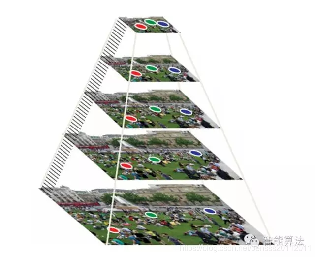
然而图像金字塔缺乏尺度的特性，因此诞生出了高斯金子塔。
高斯金字塔的尺度表达是通过不同σ的高斯函数来对图像进行卷积（即对图像做高斯平滑）:
$$L(x,y,\sigma )=G(x,y,\sigma )\ast I(x,y)$$其中G(x, y, σ) 是高斯核函数，I(x, y, σ)为输入图像
$$G(x,y,\sigma )=\frac{1}{2\pi {\sigma }^2}{e}^{\frac{x^2+y^2}{2{\sigma }^2}}$$在构建高斯金子塔的时候，有组和层之分：
1.组(o)为类似图像金字塔的层数，也就是图片是长宽按$\frac{1}{2}$进行降采样，也就是图像缩小，分辨率降低。组总数Octave
2.层(s)为组内不同σ进行高斯模糊的图片，其大小一致，一般假设组内有S层，相邻两层之间的尺度相差一个比例因子k,$k=2^{\frac{1}{S}}$,即假设上一层由$k\sigma$模糊,则接下来一层由$k^2\sigma$模糊。层总数S

由于要构成尺度连续，则上一组的倒数第三层的尺度作为下一组的第一层，后面讲完DOG金字塔时候会举例说明，可得尺度空间关系式子$$\sigma (o,s)={\sigma }_0\cdot 2^{o+\frac{s}{S}}$$
高斯金字塔构建过程
以一个512×512 512×512的图像I为例，构建高斯金字塔步骤：(从0开始计数，倒立的金字塔）
1.金字塔的组数，$(lo{g}_{2}512=9)-3$,构建的金字塔的组数为6。取每组的层数为3。
($O=lo{g}_{2}min(length,width)-a$ 一般a为3)

2.构建第0组，将图像的宽和高都增加一倍，变成1024×1024 ($I_0$)。第0层$I_0\ast G(x,y,{\sigma }_0)$，第1层$I_0\ast G(x,y,k{\sigma }_0)$，第2层$I_0\ast G(x,y,k^2{\sigma }_0)$

3.构建第1组，对$I_0$降采样变成512×512 ($I_1$)。第0层$I_1\ast G(x,y,2{\sigma }_0)$，第1层$I_1\ast G(x,y,2k{\sigma }_0)$

4.⋮ ⋮

5.构建第o组，第s层 $I_o\ast G(x,y,2^o{k}^s{\sigma }_0)$

2.DoG金字塔

由于我们需要在高斯金子塔用高斯算子进行计算LoG，但是其运算量大，转而采用DoG(差分高斯),利用差分来逼近求导方法来近似LoG。因而出现DoG金字塔，其构建过程是利用高斯金字塔的图像两两做差来得到DoG图像，你们会看到高斯金字塔每组S+3层，DoG金字塔的每组有S+2层会感到很迷。请接着看下面，等下会说清楚。
先看DoG金子塔，如图所示：

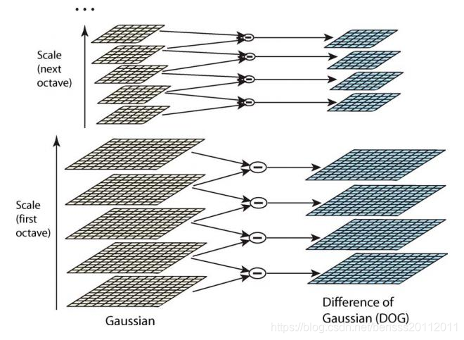
左侧的为高斯金字塔，右侧为差分金字塔，每两层高斯金字塔差分生成DoG金子塔，假设有分别$\sigma ,k\sigma$的图像做差分，即后者图像减去前者图像得出的差分为$\sigma$的图像。
知道如何生成DoG金字塔原理后，就来看看

2.1 DoG极值检测

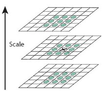
假设极值点为图中标X的位置，我们通过上一层的9个点，下一层的9个点，中间层8个点总共26个点，与X位置进行比较来检测极值。一般程序通过将这27个点组成数组，通过max与min来检测最大值与最小值。
好了，讲到这我们可以解决上面DoG金字塔为S+2层，高斯金字塔为S+3层和尺度连续性问题了。
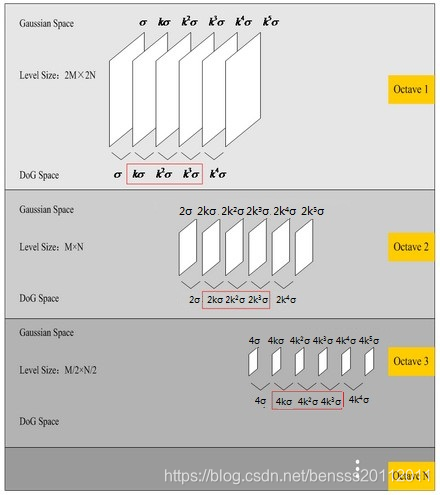
我们一般取DoG金字塔中间三层为检测的对象。这考虑到尺度连续性问题，如S = 3，则在Octave1组中$k=2^{\frac{1}{3}}$,则中间三层为$k\sigma =2^{\frac{1}{3}}\sigma ,k^2\sigma =2^{\frac{2}{3}}\sigma ,k^3\sigma =2^{\frac{3}{3}}\sigma =2\sigma$。在Octave2组中DoG的第二层$2k\sigma =2\cdot 2^{\frac{1}{3}}\sigma =2^{\frac{4}{3}}$即可看出构成尺度连续性了。而且如图所示：高斯金字塔的第一组倒数第三层$k^3\sigma$图像降采样作为第二组高斯金字塔的第一层图像，且每组第一层图像都是按这样方法得到的。
要想检测中间这三层分别的极值点，这三层最前面那一层需要上层图像，最后面一层需要下层图像。则DoG金字塔每组需要S+2层才能够检测中间三层的极值。而要想得到这S+2层DoG图像，需要高斯金字塔有S+3层图像，因为S+2层DoG图像的得到需要S+2次减法，而S+2次减法需要S+3幅图像，如图中所示：

2.2 删除不好的极值点

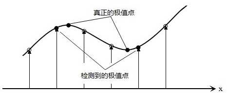
由于我们检测的极值点是在离散空间进行的，因此其极值点不一定是真正意义的极值点，我们可以从一维图像看出,我们在曲线上抽取离散点，离散点的极值点与该曲线的真正的极值点，因而我们要做曲线拟合做极值点求解。基本思想：通过泰勒公式来求解极值点。

在一维情况下，泰勒公式在$x_0$处附近展开至二阶为：
$$f(x)=f(x_0)+f^{\prime }(x_0)(x-x_0)+\frac{f^{\prime \prime }(x_0)}{2}(x-x_0{)}^2$$
在多维情况下，假设候选特征点x，其偏移量定义为Δx Δx，其对比度为D(x)的绝对值$\mid D(x)\mid$，对D(x)应用泰勒展开式:
$$D(x)=D+\frac{\partial D^T}{\partial x}\Delta x+\frac{1}{2}\Delta x^T\frac{{\partial }^{2}D}{\partial x^2}\Delta x$$
一般，$\frac{\partial D^T}{\partial x}$用J表示，为雅可比矩阵，$\frac{{\partial }^{2}D}{\partial x^2}$为H表示，为海森矩阵。上述只是简化形式，下面是将矩阵展开：
$$D(\Delta x,\Delta y,\Delta \sigma )=D(x,y,\sigma )+\left[\begin{array}{ccc}\frac{\partial D}{x}& \frac{\partial D}{y}& \frac{\partial D}{\sigma }\end{array}\right]\left[\begin{array}{c}\Delta x\\ \Delta y\\ \Delta \sigma \end{array}\right]+\frac{1}{2}\left[\begin{array}{ccc}\Delta x& \Delta y& \Delta \sigma \end{array}\right]\left[\begin{array}{ccc}\frac{{\partial }^{2}D}{\partial x^2}& \frac{{\partial }^{2}D}{\partial x\partial y}& \frac{{\partial }^{2}D}{\partial x\partial \sigma }\\ \frac{{\partial }^{2}D}{\partial y\partial x}& \frac{{\partial }^{2}D}{\partial y^2}& \frac{{\partial }^{2}D}{\partial y\partial \sigma }\\ \frac{{\partial }^{2}D}{\partial \sigma \partial x}& \frac{{\partial }^{2}D}{\partial \sigma \partial y}& \frac{{\partial }^{2}D}{\partial {\sigma }^2}\end{array}\right]\left[\begin{array}{c}\Delta x\\ \Delta y\\ \Delta \sigma \end{array}\right]$$
我们利用其简化形式，由于极值点可利用一阶导数为0来求得，因此，对简化的公式两边求导，整合后可得
$$\Delta x=-\frac{{\partial }^2{D}^{-1}}{\partial x^2}\frac{\partial D(x)}{\partial x}=-H^{-1}J$$
矩阵求导参考这个网站： https://en.wikipedia.org/wiki/Matrix_calculus#Scalar-by-vector_identities

2.3 删除边缘效应

只删除DoG响应值低的点往往是不够，一旦特征点落在图片边缘，这些点往往是不稳点的，且受噪声干扰变得不稳定。
在一个平坦的DoG响应峰值在横跨边缘有较大的主曲率，而垂直边缘方向有较小的主曲率。主曲率可通过2X2的Hessian矩阵求得:
$$H(x,y)=\left[\begin{array}{cc}{D}_{xx}(x,y)& D_{xy}(x,y)\\ D_{xy}(x,y)& D_{yy}(x,y)\end{array}\right]$$
其中，$D_{xx},D_{xy},D_{yy}$通过候选点进行差分得到的。
为了避免求具体特征值。我们先假设H的最大特征值为$\alpha$,最小特征值为$\beta$,则
$$Tr(H)=D_{xx}+D_{yy}=\alpha +\beta$$
$$Det(H)=D_{xx}+D_{yy}-D_{xy}^2=\alpha \beta$$
其中，Tr(H)为矩阵H的迹，Det(H)为矩阵H的行列式。
设$\gamma =\frac{\alpha }{\beta }$来表示最大特征值和最小特征值的比值，则
$$\frac{Tr(H{)}^2}{Det(H)}=\frac{(\alpha +\beta {)}^2}{\alpha \beta }=\frac{(\gamma \beta +\beta {)}^2}{\gamma {\beta }^2}=\frac{(\gamma +1{)}^2}{\gamma }$$
通过上面的式子，我们可以设置一个阈值$T_{\gamma }$，来检测主曲率是否在某个阈值下。
$$\frac{Tr(H{)}^2}{Det(H)}<\frac{(\gamma +1{)}^2}{\gamma }$$
上式成立，则保留特征点。(Lowe的论文给出$\gamma =10$)

3.特征点方向

当我们确定特征点后，以特征点为中心，$3\times 1.5\sigma$为半径进行直方图统计。
计算半径内每个点(x,y)的梯度的幅值（也就是模）$m(x,y)$,及方向$\theta (x,y)$，由以下两个公式决定
$$m(x,y)=\sqrt{[L(x+1,y)-L(x-1,y){]}^2+[L(x,y+1)-L(x,y-1){]}^2)}$$
$$\theta (x,y)=\arctan \frac{L(x,y+1)-L(x,y-1)}{L(x+1,y)-L(x-1,y)}$$
计算完梯度方向后，使用直方图统计特征点邻域内像素对应的梯度幅值和方向。在直方图中，不是精确的方向，而是将360°分成10份，每个相邻方向相隔36°，通过上述计算方向来近似到某个我们划分方向。（有时候360°会分成8份，每个相邻方向相隔45°）。为了得到精确方向，采用插值拟合来使方向更加精确。由于本人后面的原理还没能够理解并实现代码，用了近似原则处理了一下。有大概的实验现象，后续会跟进。

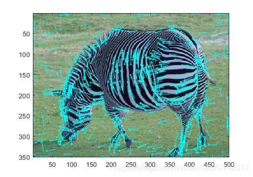
%sift文件
image = imread('animal.jpg');
image2 = image;
[Irows, Icols, channels] = size(image);
if(channels == 3)
    image = rgb2gray(image);%变成灰度图像
end
I = double(image);
%Scale space peak selection
Sigma = 1.6;
k = 2^(1/3);
DOG_Times = 4;
Octaves = 3;
Octave_outputs = ScaleSpace(I, DOG_Times, Octaves, Sigma, k);
%Detection
counter = 1;
r_tr = 10;
OriBins = 36;
winfactor = 1.5;
for i = 1:Octaves
    for j = 1:DOG_Times
        if(j ~= DOG_Times && j ~= 1)
            current = Octave_outputs(i).DOG{j}.DOG;
            below = Octave_outputs(i).DOG{j-1}.DOG;
            above = Octave_outputs(i).DOG{j+1}.DOG;
            L = Octave_outputs(i).DOG{j}.L1;
            S = Octave_outputs(i).DOG{j}.S;
            [rows, cols] = size(Octave_outputs(i).DOG{j}.DOG);
            for r = 1:rows
                for c = 1:cols
                    %avoid edges 
                    if(c ~= 1 && c ~= cols && r ~= 1 && r ~= rows)
                        X = [current(r,c) current(r + 1,c) current(r - 1,c) current(r,c + 1) current(r,c - 1) current(r + 1,c + 1) current(r - 1,c - 1) current(r + 1,c - 1) current(r - 1,c + 1) below(r,c)   below(r + 1,c)   below(r - 1,c)   below(r,c + 1)   below(r,c - 1)   below(r + 1,c + 1)   below(r - 1,c - 1)   below(r + 1,c - 1)   below(r - 1,c + 1) above(r + 1,c)   above(r - 1,c)   above(r,c + 1)   above(r,c - 1)   above(r + 1,c + 1)   above(r - 1,c - 1)   above(r + 1,c - 1)   above(r - 1,c + 1)];
                        %peak detection
                        [max_X, index_X_max] = max(X);
                        [min_X, index_X_min] = min(X);
                        if(index_X_max == 1 || index_X_min == 1)
                            if(index_X_max == 1)
                                D = max_X;
                            else
                                D = min_X;
                            end
                            Dx = (current(r,c + 1) - current(r,c - 1))/2;
                            Dy = (current(r + 1,c) - current(r - 1,c))/2;
                            Ds = (above(r,c) - below(r,c))/2;
                            D_firstDerivation = [Dx; Dy; Ds];
                            Dxx = current(r, c - 1) - 2 * current(r, c) + current(r, c + 1);
                            Dyy = current(r - 1, c) - 2 * current(r, c) + current(r + 1, c);
                            Dss = below(r, c) - 2 * current(r, c) + above(r, c);
                            Dxy = ((current(r + 1, c + 1) - current(r + 1, c - 1)) - (current(r - 1, c + 1) - current(r - 1, c - 1))) / 4;
                            Dxs = ((above(r, c + 1) - above(r, c - 1)) - (below(r, c + 1) - below(r, c - 1))) / 4;
                            Dys = ((above(r + 1, c) - above(r - 1, c)) - (below(r + 1, c) - below(r - 1, c))) / 4;
                            D_secondDerivation = [Dxx Dxy Dxs;Dxy Dyy Dys;Dxs Dys Dss];  
                            extremum_vector = -inv(D_secondDerivation) * D_firstDerivation; %extremun_vector (Δx,Δy,Δs) s: scale
                            x = c;
                            y = r;
                            s = j;
                            %使用阈值处理
                            if(extremum_vector(1) > 0.5 && ceil(c + extremum_vector(1)) < cols)
                                extremum_vector(1) = ceil( x + extremum_vector(1));
                                x = extremum_vector(1);
                            end
                            if(extremum_vector(2) > 0.5 && ceil(r + extremum_vector(2)) < rows)
                                extremum_vector(2) = ceil(y + extremum_vector(2));
                                y = extremum_vector(2);
                            end
                            if(extremum_vector(3) > 0.5 && ceil(j + extremum_vector(3)) <= DOG_Times)
                                extremum_vector(3) = ceil(s + extremum_vector(3));
                                s = extremum_vector(3);
                                L = Octave_outputs(i).DOG{s}.L1;
                                S = Octave_outputs(i).DOG{s}.S;
                            end
                            D_extremum = D + 0.5 * transp(D_firstDerivation) * extremum_vector;
                            %这里col为x，row为y
                            Dxx = current(y, x - 1) - 2 * current(y, x) + current(y, x + 1);
                            Dyy = current(y - 1, x) - 2 * current(y, x) + current(y + 1, x);
                            Dxy = ((current(y+1,x+1) - current(y+1,x-1)) - (current(y-1,x+1) - current(y-1,x-1))) / 4;
                            if(abs(D_extremum) >= (0.03 * 255))
                                H = [Dxx Dxy;Dxy Dyy];
                                if((trace(H).^2) / det(H) < ((r_tr + 1).^2) / r_tr)
                                    sigma = winfactor * Sigma * (2.^(s/k));
                                    radius = round(3 * sigma);
                                    hist = zeros(1, OriBins);
                                    %angle = atan((L(y, x + 1) - L(y, x - 1)) / L(y + 1,x) - L(y - 1, x));
                                    %特征点检测
                                    for new_r = y - radius : y + radius
                                        for new_c = x - radius : x + radius
                                            if(new_r > 1 && new_c > 1 && new_r < rows -2 && new_c < cols - 2)
                                                m = sqrt(power(L(new_r + 1, new_c) - L(new_r - 1, new_c), 2) + power(L(new_r, new_c + 1) - L(new_r, new_c - 1), 2));
                                                distance_2 = (y - new_r).^2 + (x - new_c).^2;
                                                if( m > 0.0 && distance_2 < radius * radius + 0.5)
                                                    weight = exp(- distance_2 / (2.0 * sigma * sigma));
                                                    angle = atan((L(new_r, new_c + 1) - L(new_r, new_c - 1)) / (L(new_r + 1, new_c) - L(new_r - 1, new_c)));
                                                    bin = ceil(OriBins * (angle + pi + 0.001) / ( 2.0 * pi));
                                                    bin = min(bin, OriBins);
                                                    hist(bin) = hist(bin) + m * weight;
                                                end
                                            end
                                        end
                                    end
                                    [~, index] = max(hist);
                                    angle = 2 * pi * index / OriBins;
                                    temp_Peaks(counter) = struct('r_peak',y, 'c_peak',x, 'i_octave',i, 'ori', angle, 'S',S);
                                    counter = counter + 1;
                                end
                            end
                        end
                    end
                end
            end
        end
    end
end
%将特征向量整合
for i = 1:length(temp_Peaks)
    c = temp_Peaks(i).c_peak * power(2, temp_Peaks(i).i_octave - 1);
    r = temp_Peaks(i).r_peak * power(2,temp_Peaks(i).i_octave - 1);
    locs(i,:) = [r c temp_Peaks(i).S temp_Peaks(i).ori];
end

image = image2;
computer_feature = counter - 1
showkeys(image, locs);

%金字塔构建
function Octave_outputs = ScaleSpace( I_input, DOG_Times, Octaves, Sigma,k)
%I_input: the orginal input Image
%DOG_Times: the number of times that Difference of Gaussian should be computed
%Octaves: How many octaves should be computed
%Sigma: is the sigma value for Gaussain filter
%k: is the scale value that will be multiplied by sigma to compute the Gaussian and find DOG

DOG = cell(1,DOG_Times);
counter = 0;

for j = 1:Octaves
    %First Gaussian Filter
    GaussainSize = ceil(7*(Sigma * (k^counter)));%一般高斯核的大小在6倍方差，这里可以改成6
    H = fspecial('gaussian' , [GaussainSize,GaussainSize ], Sigma * (k^counter));%建立每组第一个高斯核
    if(j > 1)
        I_input = I_input(1:2:end,1:2:end);%缩小图片尺寸
    end
    for i = 1:DOG_Times
        L1 = conv2(I_input, H, 'same');
        GaussainSize = ceil(7*(Sigma*(k^(i+counter))));
        H = fspecial('gaussian' , [GaussainSize,GaussainSize ], Sigma * (k^(i+counter)));
        L2 = conv2(I_input, H, 'same');
        %DOG and save it
        Octave_outputs(j).DOG{i} = struct('DOG', L2 - L1, 'L2', L2, 'L1', L1, 'S', Sigma*(k^(i+counter)));
    end
    counter = counter + 1;
end
end

展示特征点，引用sift论文
% showkeys(image, locs)
%
% This function displays an image with SIFT keypoints overlayed.
%   Input parameters:
%     image: the file name for the image (grayscale)
%     locs: matrix in which each row gives a keypoint location (row,
%           column, scale, orientation)

function showkeys(image, locs)

disp('Drawing SIFT keypoints ...');

% Draw image with keypoints
figure('Position', [50 50 size(image,2) size(image,1)]);
colormap('gray');
imagesc(image);
hold on;
imsize = size(image);
for i = 1: size(locs,1)
    % Draw an arrow, each line transformed according to keypoint parameters.
    TransformLine(imsize, locs(i,:), 0.0, 0.0, 1.0, 0.0);
    TransformLine(imsize, locs(i,:), 0.85, 0.1, 1.0, 0.0);
    TransformLine(imsize, locs(i,:), 0.85, -0.1, 1.0, 0.0);
end
hold off;


% ------ Subroutine: TransformLine -------
% Draw the given line in the image, but first translate, rotate, and
% scale according to the keypoint parameters.
%
% Parameters:
%   Arrays:
%    imsize = [rows columns] of image
%    keypoint = [subpixel_row subpixel_column scale orientation]
%
%   Scalars:
%    x1, y1; begining of vector
%    x2, y2; ending of vector
function TransformLine(imsize, keypoint, x1, y1, x2, y2)

% The scaling of the unit length arrow is set to approximately the radius
%   of the region used to compute the keypoint descriptor.
len = 6 * keypoint(3);

% Rotate the keypoints by 'ori' = keypoint(4)
s = sin(keypoint(4));
c = cos(keypoint(4));

% Apply transform
r1 = keypoint(1) - len * (c * y1 + s * x1);
c1 = keypoint(2) + len * (- s * y1 + c * x1);
r2 = keypoint(1) - len * (c * y2 + s * x2);
c2 = keypoint(2) + len * (- s * y2 + c * x2);

line([c1 c2], [r1 r2], 'Color', 'c');

参考链接

https://wenku.baidu.com/view/87270d2c2af90242a895e52e.html?re=view
https://www.cnblogs.com/ronny/p/4028776.html
https://www.cnblogs.com/wangguchangqing/p/4853263.html#autoid-4-2-0
https://blog.youkuaiyun.com/dcrmg/article/details/52561656
https://www.cnblogs.com/JiePro/p/sift_1.html

如有错误，请大家指出，谢谢。