


 本文通过Python的statsmodels库计算了Anscombe四组数据集的x与y的均值、方差及相关系数,并利用Seaborn进行了可视化展示。同时使用线性回归分析了各数据集间的联系。
Part 1
For each of the four datasets…
- Compute the mean and variance of both x and y
- Compute the correlation coefficient between x and y
- Compute the linear regression line: y=β0+β1x+ϵ (hint: use statsmodels and look at the Statsmodels notebook)
Part 2
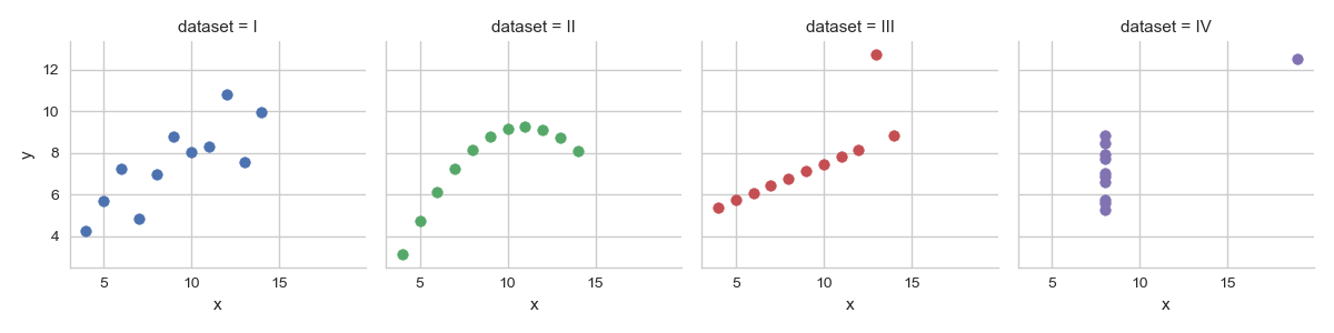
Using Seaborn, visualize all four datasets.
hint: use sns.FacetGrid combined with plt.scatte
import pandas as pd
import seaborn as se
import matplotlib.pyplot as plt
import statsmodels.api as st
ans = se.load_dataset('anscombe')
df = ans.groupby('dataset')
mean_var = pd.concat([df.mean(), df.var()], keys=['mean', 'variance'])
corr = pd.concat([df.corr()], keys=['correlation'])
print(mean_var)
print(corr)

data_dict = dict(list(df))
array_x, array_y = {}, {}
for key, value in data_dict.items():
    array_x[key] = value['x'].values
    array_y[key] = value['y'].values
for key in array_x.keys():
    x = st.add_constant(array_x[key])
    y = array_y[key]
    est = st.OLS(y, x).fit()
    params = est.params
    print(key, ': beta0 =', params[0], 'beta1 =', params[1])
se.set(style='whitegrid')
g = se.FacetGrid(ans, col="dataset", hue="dataset")
g.map(plt.scatter, 'x', 'y')
plt.show()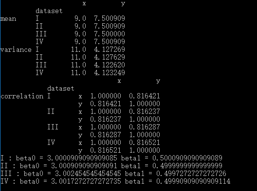


 824
824

 被折叠的 条评论
为什么被折叠?
被折叠的 条评论
为什么被折叠?
 到【灌水乐园】发言


