01-线性回归sklearn实现

一、传统方式绘制直线并计算斜率

（1）绘制一条直线

（2）已知两点，绘制一条直线

（3）已知两点，求直线斜率

二、利用sklearn线性回归求直线斜率

sklearn.linear_model.LinearRegression

sklearn.datasets.make_regression

三、糖尿病数据集的线性回归分析

四、岭回归的参数调节

参数调节

岭迹分析-模型系数的可视化比较

五、LASSO回归

LASSO回归的参数调节

一、传统方式绘制直线并计算斜率

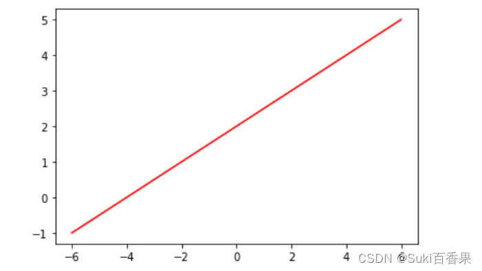
（1）绘制一条直线

%matplotlib inline
import numpy as np
import matplotlib.pyplot as plt
x=np.linspace(-6,6,100)
y=0.5*x+2
plt.figure()
plt.plot(x,y,color='red')
plt.show()

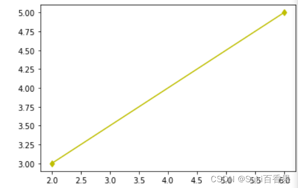
（2）已知两点，绘制一条直线

x=np.array([2,6])
y=np.array([3,5])
plt.plot(x,y,'yd-')
plt.show()

（3）已知两点，求直线斜率

k=(y[1]-y[0])/(x[1]-x[0])
print(k)

二、利用sklearn线性回归求直线斜率

sklearn.linear_model.LinearRegression

LinearReagression(
'fit_intercept=True'  #节距是否使用

'normalize=False'   #标准化

'copy_x=True'         #复制x,是否覆盖原始的x

'n_jobs=None'        #计算时设置的任务个数（-1表示使用所有的CPU）

)#大部分取默认值

属性

coef_         输出系数，没有截距

intercept_  输出截距

rank_         输出矩阵的秩

singular     矩阵X的奇异值，仅在x为密集矩阵时有效

方法

fit(self,X,y[,sample_weight])         #训练模型，sample_weight为每个样本的权重值

predict(self,X)                               #模型预测，返回预测值

score(self,X,y['sample_weight])    #模型pinggu，放回R^2系数，最优质为1，说明所有数据都预测正确

get_params（self['deep]）           #deep默认为True，返回超参数的值

set_params(self.** params)          #修改超参数的值
 

利用线性回归求通过平面上两点（2,3）（6,5）的直线斜率

#利用线性回归求通过平面上两点（2,3）（6,5）的直线斜率
from sklearn.linear_model import LinearRegression
x=np.array([2,6])
y=np.array([3,5])
x=x.reshape(-1,1)
#实例化
lr=LinearRegression()
lr.fit(x,y)
print("过两点(2,3)与(6,5)的直线斜率为:{},截距项为:{:.2f}".format(lr.coef_,lr.intercept_))

Out：过两点(2,3)与(6,5)的直线斜率为:[0.5],截距项为:2.00

#模型预测
x_test=np.array([3,4,5]).reshape(-1,1)
y_predict=lr.predict(x_test)
y_predict

Out：array([3.