PyTorch深度学习实践：从分类到生成-PyTorch构建CIFAR10分类器-优快云博客

训练分类器

学习目标

在本课程中，我们将使用 CIFAR10 数据集。通过本课程可以了解到定义、训练、测试分类器的过程。

学习内容

1. 使用CIFAR10 数据集训练分类器

1.1 导包

%matplotlib inline

import torch
import torchvision
import torchvision.transforms as transforms

torchvision 数据集的输出是范围 [0， 1] 的 PILImage 图像。将它们转换为归一化范围 [-1， 1] 的 Tensor。

1.2 加载数据

!wget https://model-community-picture.obs.cn-north-4.myhuaweicloud.com/ascend-zone/notebook_datasets/0bae26b00e9711f095dcfa163edcddae/data.zip

!unzip data.zip

加载,预处理CIFAR-10数据集，创建训练和测试的数据加载器，并定义了数据集中的类别名称。

transform = transforms.Compose(
    [transforms.ToTensor(),
     transforms.Normalize((0.5, 0.5, 0.5), (0.5, 0.5, 0.5))])

batch_size = 4

trainset = torchvision.datasets.CIFAR10(root='./data', train=True,
                                        download=True, transform=transform)
trainloader = torch.utils.data.DataLoader(trainset, batch_size=batch_size,
                                          shuffle=True, num_workers=2)

testset = torchvision.datasets.CIFAR10(root='./data', train=False,
                                       download=True, transform=transform)
testloader = torch.utils.data.DataLoader(testset, batch_size=batch_size,
                                         shuffle=False, num_workers=2)

classes = ('plane', 'car', 'bird', 'cat',
           'deer', 'dog', 'frog', 'horse', 'ship', 'truck')

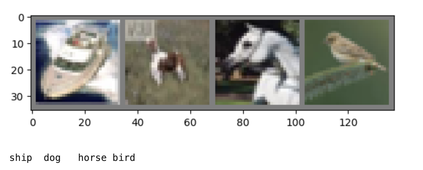
展示部分训练图片

import matplotlib.pyplot as plt
import numpy as np
import torchvision

# 显示图像的功能
def imshow(img):
    img = img / 2 + 0.5     # unnormalize
    npimg = img.numpy()
    plt.imshow(np.transpose(npimg, (1, 2, 0)))
    plt.show()

# 得到一些随机的训练图片
dataiter = iter(trainloader)
images, labels = next(dataiter) 
# 展示图片
imshow(torchvision.utils.make_grid(images))

# 打印类别
print(' '.join(f'{classes[labels[j]]:5s}' for j in range(len(labels))))

在这里插入图片描述

1.3 定义卷积神经网络

import torch.nn as nn
import torch_npu
import torch.nn.functional as F

device = torch.device("npu:0" if torch.npu.is_available() else "cpu")
torch_npu.npu.set_device(device)


class Net(nn.Module):
    def __init__(self):
        super().__init__()
        self.conv1 = nn.Conv2d(3, 6, 5)
        self.pool = nn.MaxPool2d(2, 2)
        self.conv2 = nn.Conv2d(6, 16, 5)
        self.fc1 = nn.Linear(16 * 5 * 5, 120)
        self.fc2 = nn.Linear(120, 84)
        self.fc3 = nn.Linear(84, 10)

    def forward(self, x):
        x = self.pool(F.relu(self.conv1(x)))
        x = self.pool(F.relu(self.conv2(x)))
        x = torch.flatten(x, 1) # flatten all dimensions except batch
        x = F.relu(self.fc1(x))
        x = F.relu(self.fc2(x))
        x = self.fc3(x)
        return x


net = Net().to(device)

1.4 定义损失函数和优化器

使用 Classification Cross-Entropy 损失和带有动量的 SGD。

import torch.optim as optim

criterion = nn.CrossEntropyLoss()
optimizer = optim.SGD(net.parameters(), lr=0.001, momentum=0.9)

1.5 训练网络

遍历数据迭代器，并将输入馈送到网络并进行优化。

for epoch in range(2):  # 多次遍历数据集
    running_loss = 0.0
    for i, data in enumerate(trainloader, 0):
        # 获取输入；数据是一个 [输入，标签] 的列表
        inputs, labels = data[0].to(device), data[1].to(device)

        # zero the parameter gradients
        optimizer.zero_grad()

        # forward + backward + optimize
        outputs = net(inputs)
        loss = criterion(outputs, labels)
        loss.backward()
        optimizer.step()

        # print statistics
        running_loss += loss.item()
        if i % 2000 == 1999:    # 每2000个小批量打印一次
            print(f'[{epoch + 1}, {i + 1:5d}] loss: {running_loss / 2000:.3f}')
            running_loss = 0.0

print('Finished Training')

out：

[1, 2000] loss: 2.181
[1, 4000] loss: 1.835
[1, 6000] loss: 1.658
[1, 8000] loss: 1.576
[1, 10000] loss: 1.518
[1, 12000] loss: 1.481
[2, 2000] loss: 1.396
[2, 4000] loss: 1.375
[2, 6000] loss: 1.357
[2, 8000] loss: 1.344
[2, 10000] loss: 1.313
[2, 12000] loss: 1.282
Finished Training

保存经过训练的模型：

PATH = './cifar_net.pth'
torch.save(net.state_dict(), PATH)

1.6 在测试数据上测试网络

刚刚已经在训练数据集上训练了2轮。需要检查网络是否学到了任何东西。
通过预测神经网络输出的类标签，并根据真实值进行检查。如果预测正确，将样本添加到正确预测列表中。
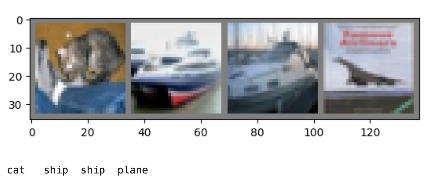
展示测试集中的部分图像。

dataiter = iter(testloader)

images, labels = next(dataiter)

imshow(torchvision.utils.make_grid(images))
print(' '.join(f'{classes[labels[j]]:5s}' for j in range(len(labels))))

在这里插入图片描述

重新加载已保存的模型（注意：这里不需要保存和重新加载模型，只是为了展示如何做到这一点）：

net = Net().to(device)
net.load_state_dict(torch.load(PATH))

labels = labels.to(device)
images = images.to(device)

outputs = net(images)

查看预测结果：

_, predicted = torch.max(outputs, 1)

print('Predicted: ', ' '.join(f'{classes[predicted[j]]:5s}'
                              for j in range(4)))

Out:

Predicted: frog ship car ship

测试网络在整个数据集上的表现如何。

# 测试模型
correct = 0
total = 0
# 因为没有训练，所以不需要计算输出的梯度
with torch.no_grad():
    for data in testloader:
        images, labels = data
        # 将数据移动到 NPU 设备
        labels = labels.to(device)
        images = images.to(device)
        # 通过将图像输入网络来计算输出
        outputs = net(images)
        # 预测的类别是得分最高的类别
        _, predicted = torch.max(outputs.data, 1)
        total += labels.size(0)
        correct += (predicted == labels).sum().item()

print(f'Accuracy of the network on the 10000 test images: {100 * correct // total} %')

Out:
Accuracy of the network on the 10000 test images: 55 %

这看起来比偶然性要好得多，偶然性是 10% 的准确率（从 10 个类别中随机选择一个类别）。似乎网络学到了一些东西。

表现良好的类有哪些，表现不佳的类有哪些：

# 准备为每个类别计算预测值
correct_pred = {classname: 0 for classname in classes}
total_pred = {classname: 0 for classname in classes}


# 不需要梯度
with torch.no_grad():
    for data in testloader:
        images, labels = data
        images = images.to(device)
        outputs = net(images)
        _, predictions = torch.max(outputs, 1)
        # 得到每个类的正确预测
        for label, prediction in zip(labels, predictions):
            if label == prediction:
                correct_pred[classes[label]] += 1
            total_pred[classes[label]] += 1


# 打印每个类别的正确率
for classname, correct_count in correct_pred.items():
    accuracy = 100 * float(correct_count) / total_pred[classname]
    print(f'Accuracy for class: {classname:5s} is {accuracy:.1f} %')

out:

Accuracy for class: plane is 52.9 %
Accuracy for class: car is 68.2 %
Accuracy for class: bird is 32.2 %
Accuracy for class: cat is 44.3 %
Accuracy for class: deer is 48.4 %
Accuracy for class: dog is 41.3 %
Accuracy for class: frog is 69.6 %
Accuracy for class: horse is 55.1 %
Accuracy for class: ship is 69.1 %
Accuracy for class: truck is 69.5 %