计算物理（浮点数精度相关）

来源：

  某次计算物理作业（我不能接受不放出完整代码）

题目：

代码：

import matplotlib.pyplot as plt
import numpy as np
from mpmath import mp

# 设置mpmath库的精度为四倍精度
mp.dps = 36


# 定义函数
def func(x):
    return (x - 1) ** 12


def func2(x):
    return x ** 12 - 12 * x ** 11 + 66 * x ** 10 - 220 * x ** 9 + 495 * x ** 8 - 792 * x ** 7 + 924 * x ** 6 - 792 * x ** 5 + 495 * x ** 4 - 220 * x ** 3 + 66 * x ** 2 - 12 * x + 1


def func3(x):
    return (((((((((((
                             x - 12) * x + 66) * x - 220) * x + 495) * x - 792) * x + 924) * x - 792) * x + 495) * x - 220) * x + 66) * x - 12) * x + 1


# 定义 x 范围
x_single = np.linspace(0.998, 1.002, 400, dtype=np.float32)
x_double = np.linspace(0.998, 1.002, 400, dtype=np.float64)
step = mp.mpf('0.00001')
x_quad = [mp.mpf(val) for val in mp.arange('0.998', '1.002', step)]

# 计算函数值
y_single = func(x_single)
y_double = func(x_double)
y_quad = [func(x) for x in x_quad]

# 计算展开式函数图
y_single2 = func2(x_single)
y_double2 = func2(x_double)
y_quad2 = [func2(x) for x in x_quad]
y_single3 = func3(x_single)
y_double3 = func3(x_double)
y_quad3 = [func3(x) for x in x_quad]

# 绘制图像
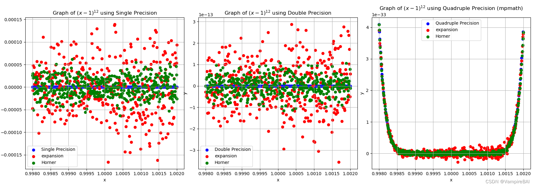
plt.figure(figsize=(24, 6))

plt.subplot(1, 3, 1)
plt.scatter(x_single, y_single, label='Single Precision', color='blue')
plt.scatter(x_single, y_single2, label='expansion', color='red')
plt.scatter(x_single, y_single3, label='Horner', color='green')
plt.xlabel('x')
plt.ylabel('y')
plt.legend()
plt.grid(True)
plt.title('Graph of $(x-1)^{12}$ using Single Precision')

plt.subplot(1, 3, 2)
plt.scatter(x_double, y_double, label='Double Precision', color='blue')
plt.scatter(x_double, y_double2, label='expansion', color='red')
plt.scatter(x_single, y_double3, label='Horner', color='green')
plt.xlabel('x')
plt.ylabel('y')
plt.legend()
plt.grid(True)
plt.title('Graph of $(x-1)^{12}$ using Double Precision')

plt.subplot(1, 3, 3)
plt.scatter(x_quad, y_quad, label='Quadruple Precision', color='blue')
plt.scatter(x_quad, y_quad2, label='expansion', color='red')
plt.scatter(x_single, y_quad3, label='Horner', color='green')
plt.xlabel('x')
plt.ylabel('y')
plt.legend()
plt.grid(True)
plt.title('Graph of $(x-1)^{12}$ using Quadruple Precision (mpmath)')

plt.tight_layout()
plt.show()

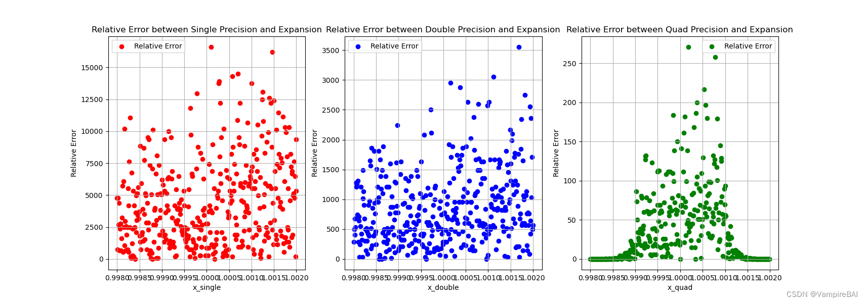
# 设置一个很小的数，用于替代零
epsilon_single = 1e-8
epsilon_double = 1e-16
epsilon_quad = 1 * 10 ** (-36)

# 计算相对误差，避免除以零
relative_error_single = np.abs(y_single - y_single2) / (np.abs(y_single) + epsilon_single)
relative_error_double = np.abs(y_double - y_double2) / (np.abs(y_double) + epsilon_double)
y_quad = np.array(y_quad)
y_quad2 = np.array(y_quad2)
relative_error_quad = np.abs(y_quad - y_quad2) / (np.abs(y_quad) + epsilon_quad)

# 绘制相对误差图表
plt.figure(figsize=(24, 6))
plt.subplot(1, 3, 1)
plt.scatter(x_single, relative_error_single, label='Relative Error', color='red')
plt.xlabel('x_single')
plt.ylabel('Relative Error')
plt.legend()
plt.grid(True)
plt.title('Relative Error between Single Precision and Expansion')

plt.subplot(1, 3, 2)
plt.scatter(x_double, relative_error_double, label='Relative Error', color='blue')
plt.xlabel('x_double')
plt.ylabel('Relative Error')
plt.legend()
plt.grid(True)
plt.title('Relative Error between Double Precision and Expansion')

plt.subplot(1, 3, 3)
plt.scatter(x_quad, relative_error_quad, label='Relative Error', color='green')
plt.xlabel('x_quad')
plt.ylabel('Relative Error')
plt.legend()
plt.grid(True)
plt.title('Relative Error between Quad Precision and Expansion')

plt.show()

输出结果：

结语：

由于肉眼就可以看出改进方法后误差的缩小，所以就在误差分析图中没有再添加