python-机器学习 感知器分类算法

感知器分类算法

一、基本概念

1. 神经元的数学表示

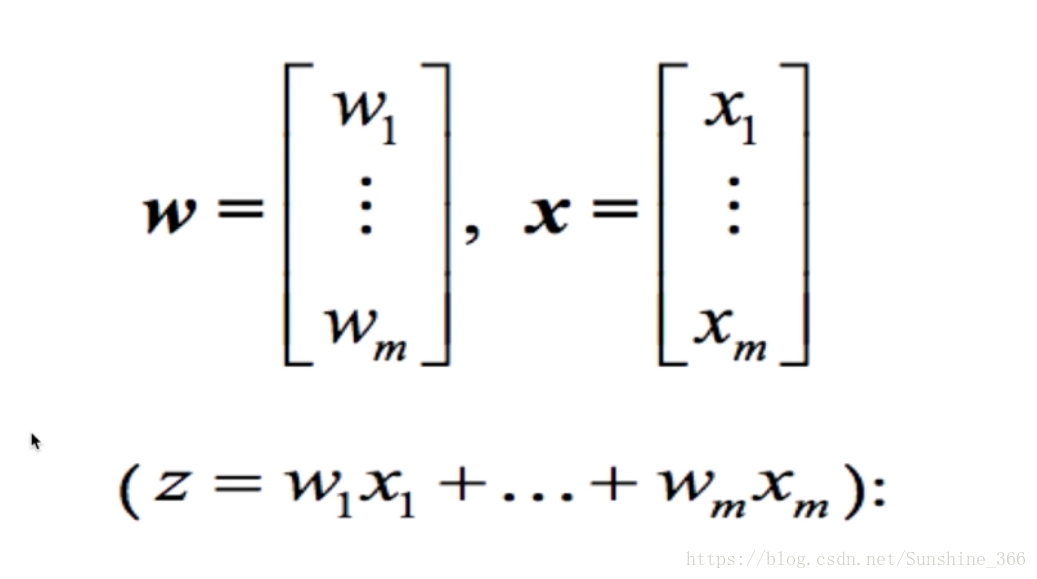
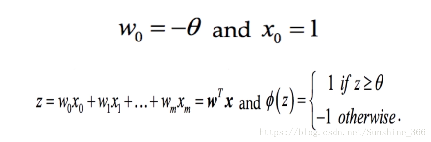
X向量组表示神经元电信号，W 向量组是弱化神经元电信号的系数组合。Z为处理后的信号。

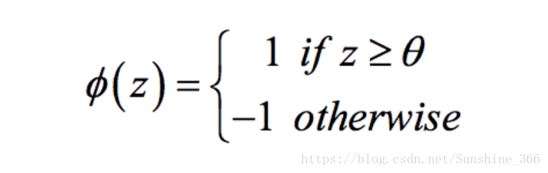
2. 激活函数

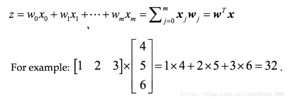
3. 向量点积

 

二、感知器分类算法

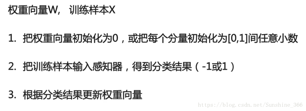
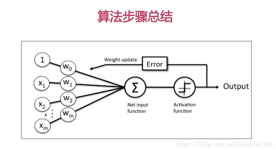
1. 感知器数据分类算法步骤

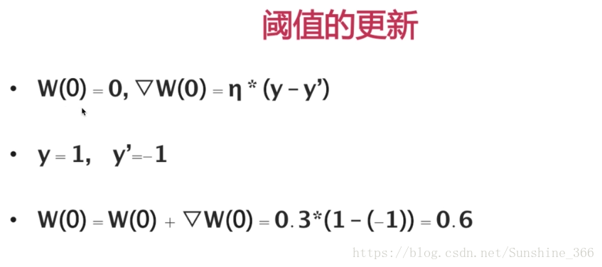
2. 步调函数阈值

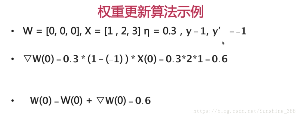
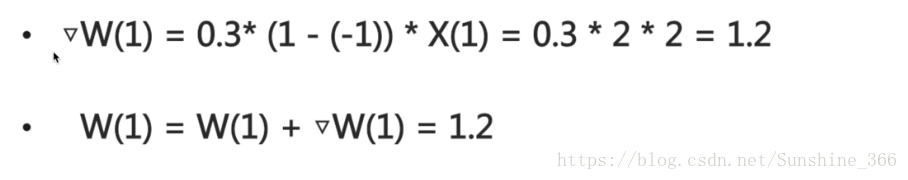
3. 权重更新算法

 

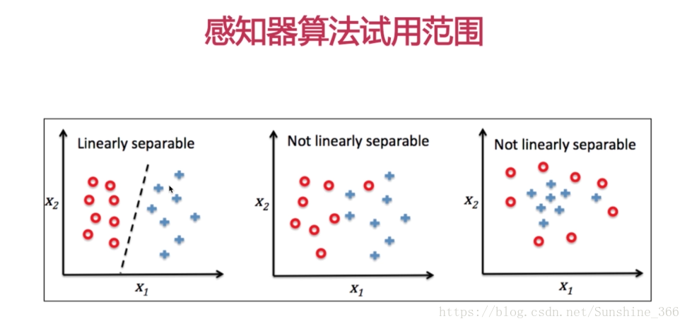
4.  适用于第一种数据样本，可线性分割。

5.

 

6.  感知器分类算法的Python实现

 感知器算法

# coding=utf-8
import numpy as np
class Perceptron(object):
    """
    eta: 学习率
    n_iter: 权重向量的训练次数
    w_: 神经分叉权重向量
    errors_: 记录神经元判断出错的次数
    """
    def __init__(self, eta=0.01, n_iter=10):
        self.eta = eta
        self.n_iter = n_iter
        pass

    def net_input(self, X):
        """
         np.dot做向量点积
        :param self:
        :param x:
        :return:
        """
        return np.dot(X, self.w_[1:]) + self.w_[0]
        pass

    def predict(self, X):
        return np.where(self.net_input(X) >= 0.0, 1, -1)
        pass

    def fit(self, X, y):
        """
        输入训练数据，培训神经元
        :param x: 输入样本向量
        x: shape[n_samples, n_features]
        :param y:对应样本分类
        ###
        x:[[1,2,3],[4,5,6]]
        n_samples: 2
        n_features: 3
        y: [1, -1]
        ###
        :return:
        """
        self.w_ = np.zeros(1 + X.shape[1])
        self.errors_ = []
        for _ in range(self.n_iter):
            errors = 0
            """
            x:[[1,2,3],[4,5,6]]
            y: [1, -1]
            zip(x, y) = [[1,2,3, 1],[4,5,6, -1]]
            """
            for xi, target in zip(X, y):
                update = self.eta * (target - self.predict(xi))
                """
                xi:是一个向量
                update * xi等价：
                [▽w(1) = x[1]*update, ▽w(2) = x[2]*update, ▽w(3) = x[3]*update, 
                """
                self.w_[1:] += update * xi
                self.w_[0] += update
                errors += int(update != 0.0)
                self.errors_.append(errors)
                pass
            pass
        pass

利用感知器算法对数据进行分类

# coding=utf-8
import pandas as pd
import matplotlib.pyplot as plt
import numpy as np
from ganzhiqi import *
from matplotlib.colors import ListedColormap
file = "C:/Users/25143/Desktop/python_test/pytdata1.csv"
df = pd.read_csv(file, header=None)
y = df.loc[0:99, 4].values
y = np.where(y == 'Iris-setosa', -1, 1)
X = df.iloc[0:100, [0, 2]].values
# print(X)
plt.scatter(X[:50, 0], X[:50, 1], color='red', marker='o', label='setosa')
plt.scatter(X[50:100, 0], X[50:100, 1], color='blue', marker='x', label='versicolor')
plt.xlabel('花瓣长度')
plt.ylabel('花茎长度')
plt.legend(loc='upper left')
plt.show()

ppn = Perceptron(eta=0.1, n_iter=10)
ppn.fit(X, y)
plt.plot(range(1, len(ppn.errors_) + 1), ppn.errors_, marker='o')
plt.xlabel('Epochs')
plt.ylabel('错误分类次数')


def plot_decision_regions(X, y, classifer, resolution=0.02):
    marker = ('s', 'x', 'o', 'v')
    colors = ('red', 'blue', 'lightgreen', 'gray', 'cyan')
    cmap = ListedColormap(colors[:len(np.unique(y))])
    x1_min, x1_max = X[:, 0].min()-1, X[:, 0].max()
    x2_min, x2_max = X[:, 1].min()-1, X[:, 1].max()
    xx1, xx2 = np.meshgrid(np.arange(x1_min, x1_max, resolution),
                           np.arange(x2_min, x2_max, resolution))
    # print(np.arange(x2_min, x2_max, resolution).shape)
    # print(np.arange(x2_min, x2_max, resolution))
    Z = classifer.predict(np.array([xx1.ravel(), xx2.ravel()]).T)
    # print(xx1.ravel())
    Z = Z.reshape(xx1.shape)
    plt.contourf(xx1, xx2, Z, alpha=0.4, cmap=cmap)
    plt.xlim(xx1.min(), xx1.max())
    plt.ylim(xx2.min(), xx2.max())
    for idx, c1 in enumerate(np.unique(y)):
         plt.scatter(x=X[y == c1, 0], y=X[y == c1, 1], alpha=0.8, c=cmap(idx),
                    marker=marker[idx], label=c1)


plot_decision_regions(X, y, ppn, resolution=0.02)
plt.xlabel('花茎长度')
plt.ylabel('花瓣长度')
plt.legend(loc='upper left')
plt.show()

 使用的数据示例

 

3.22,3.08,1.65,0.24,Iris-setosa
4.15,3.22,1.83,0.34,Iris-setosa
4.35,3.99,1.9,0.4,Iris-setosa
4.32,3.9,1.01,0.24,Iris-setosa
5.96,3.55,1.3,0.18,Iris-setosa
5.55,3.42,1.64,0.25,Iris-setosa
4.41,3.99,1.87,0.39,Iris-setosa
4.25,3.42,1.02,0.12,Iris-setosa
5.73,3.68,1.44,0.16,Iris-setosa
4.28,3.87,1.41,0.21,Iris-setosa
5.92,3.69,1.65,0.26,Iris-setosa
4.58,3.15,1.39,0.17,Iris-setosa
5.18,3.75,1.42,0.24,Iris-setosa
5.99,3.18,1.08,0.15,Iris-setosa
5.95,3.09,1.09,0.24,Iris-setosa
4.58,3.86,1.14,0.29,Iris-setosa
5.32,3.69,1.72,0.22,Iris-setosa
5.07,3.75,1.86,0.48,Iris-setosa
5.58,3.82,1.86,0.31,Iris-setosa
5.44,3.51,1.49,0.32,Iris-setosa
5.67,3.65,1.58,0.18,Iris-setosa
4.81,3.02,1.09,0.28,Iris-setosa
5.02,3.85,1.6,0.41,Iris-setosa
5.16,3.26,1.62,0.17,Iris-setosa
5.78,3.46,1.98,0.27,Iris-setosa
5.14,3.25,1.59,0.42,Iris-setosa
4.97,3.38,1.23,0.35,Iris-setosa
4.47,3.44,1.71,0.26,Iris-setosa
5.51,3.81,1.92,0.18,Iris-setosa
5.5,3.99,1.72,0.41,Iris-setosa
5.47,3.18,1.89,0.49,Iris-setosa
5.79,3.12,1.34,0.1,Iris-setosa
4.24,3.53,1.1,0.33,Iris-setosa
5.66,3.53,1.79,0.5,Iris-setosa
4.24,3.39,1.23,0.36,Iris-setosa
4.56,3.04,1.17,0.1,Iris-setosa
5.49,4,1.98,0.5,Iris-setosa
4.3,3.21,1.07,0.45,Iris-setosa
4.62,3.85,1.75,0.43,Iris-setosa
5.07,3.04,1.22,0.12,Iris-setosa
4.12,3.22,1.24,0.15,Iris-setosa
4.17,3.76,1.86,0.34,Iris-setosa
5.76,3.06,1.94,0.4,Iris-setosa
4.2,3.2,1.63,0.47,Iris-setosa
5.82,3.25,1.49,0.29,Iris-setosa
5.65,3.88,1.35,0.46,Iris-setosa
4.57,3.9,1.68,0.45,Iris-setosa
5.62,3.55,1.41,0.44,Iris-setosa
5.88,3.71,1.73,0.25,Iris-setosa
4.12,3.54,1.78,0.1,Iris-setosa
5.28,3.28,1.79,0.24,Iris-setosa
5.3,3.17,1.95,0.29,Iris-setosa
5.75,3.85,1.75,0.46,Iris-setosa
4.76,3.62,1.54,0.21,Iris-setosa
4.03,3.9,1.36,0.46,Iris-setosa
5.61,3.19,1.32,0.27,Iris-setosa
5.19,3.04,1.19,0.17,Iris-setosa
4.02,3.4,1.9,0.17,Iris-setosa
4.46,3.21,1.28,0.3,Iris-setosa
4.78,3.7,1.98,0.42,Iris-setosa
5.37,3.12,1.45,0.4,Iris-setosa
4.23,3.13,1.54,0.22,Iris-setosa
5.69,3.26,1.9,0.48,Iris-setosa
5.9,3.77,1.67,0.36,Iris-setosa
4.06,3.36,1.31,0.12,Iris-setosa
5.18,3.87,1.55,0.45,Iris-setosa
4.52,3.77,1.6,0.45,Iris
4.46,3.49,1.54,0.18,Iris
4.46,3.38,1.86,0.19,Iris
4.4,3.38,1.28,0.3,Iris
4.92,3.64,1.46,0.14,Iris
5.75,3.44,1.69,0.23,Iris
5.02,3.2,1.66,0.47,Iris
4.1,3.45,1.07,0.29,Iris
5.24,3.85,1.8,0.36,Iris
4.52,3.01,1.04,0.48,Iris
4.24,3.29,1.15,0.41,Iris
5.26,3.01,1.34,0.15,Iris
4.67,3.09,1.51,0.22,Iris
5.67,3.23,1.96,0.12,Iris
5.75,3.31,1.33,0.3,Iris
4.7,3.13,1.74,0.24,Iris
4.4,3.84,1.66,0.24,Iris
4.27,3.58,1.87,0.1,Iris
5.6,3.41,1.31,0.15,Iris
4.61,3.91,1.13,0.43,Iris
5.06,3.53,1.05,0.19,Iris
5.62,3.92,1.77,0.15,Iris
4.24,3.18,1.22,0.2,Iris
4.95,3.5,1.46,0.21,Iris
5.89,3.54,1.62,0.12,Iris
5.89,3.15,1.7,0.2,Iris
4.69,3.9,1.56,0.3,Iris
4.32,3.06,1.54,0.28,Iris
4.07,3.03,1.33,0.21,Iris
4.49,3.59,1.52,0.2,Iris
4.92,3.8,1.56,0.42,Iris
5.95,3.39,1.21,0.48,Iris
4.42,3.85,1.8,0.25,Iris
4.57,3.59,1.66,0.25,Iris