机器学习之线性回归

简单的线性回归

以某产品的温度和产率关系为例，其中产率(y)是温度(x)的函数。请构建模型预测产品产率。

温度	产率
100	45
110	51
120	54
130	61
140	66
150	70
160	74
170	78
180	85
190	89

首先，我们可以先把数据可视化，画个散点图出来。

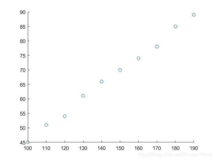
根据散点图可知，数据基本上都在一条直线上，我们可以用一条直线去拟合。

正规方程求解

$$\theta =(X^{T}X{)}^{-1}{X}^{T}Y$$

function [ theta ] = linearReg( )
% 线性回归正规方程求解
% 用130、190作为测试集
train = 8;
X = [1 100;1  110;1  120;1  140;1  150;1  160;1  170;1  180;] 
Y = [45; 51 ;54 ;66; 70; 74 ;78; 85];
A = inv(X'*X);
theta = A*X'*Y;
end

解得：
$$\theta =\left(\begin{array}{c}-3.1507\\ 0.4851\end{array}\right)$$

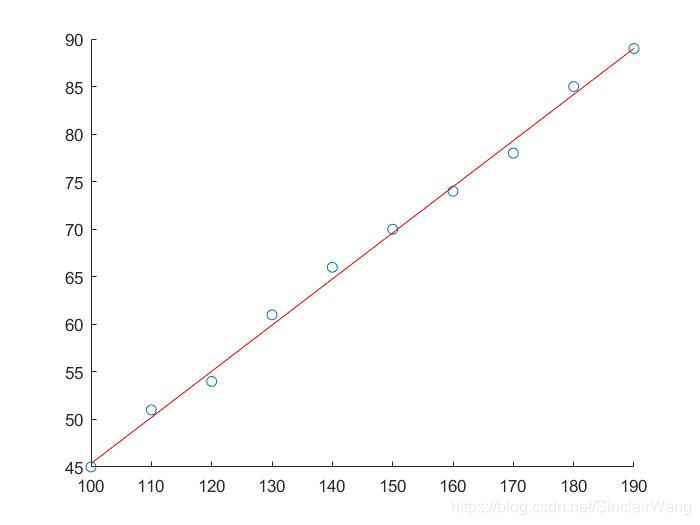
散点图拟合情况如下：

看起来拟合效果还不错

梯度下降求解

假设函数：$$h_{\theta }(x)={\theta }_0+{\theta }_{1}x$$
代价函数：
$$J({\theta }_0,{\theta }_1)=\frac{1}{2m}\sum _{i=1}^m(h_{\theta }(x^{(i)})-y^{(i)}{)}^2$$

梯度下降：(同步更新)
$$tem{p}_0={\theta }_0-\alpha \frac{\partial }{\partial {\theta }_0}J({\theta }_0,{\theta }_1)$$
$$tem{p}_1={\theta }_1-\alpha \frac{\partial }{\partial {\theta }_1}J({\theta }_0,{\theta }_1)$$
$${\theta }_0=tem{p}_0$$
$${\theta }_1=tem{p}_1$$

假设函数

function [ res ] = h_func(inputx,theta )
% 预测函数
res = theta(1)+theta(2)*inputx;
end

代价函数

function [ jVal,gradient ] = costFunction2( theta )
% jVal 为 代价值 gradient为梯度
% cost function
% 用130、190作为测试集
x = [100 110 120  140  150  160  170  180] 
y = [45 51 54 66 70 74 78 85];
m = size(x,1);  % size(x) = [1 8] size(x,1) 表示获取x的行 
hypothesis = h_func(x,theta); 
delta = hypothesis - y; % 预测误差 向量
jVal= sum(delta.^2);  % 损失函数
gradient(1) = sum(delta)/m;
gradient(2) = sum(delta.*x)/m;
end

梯度下降

function [ optTheta,functionVal,exitFlag ] = Gradient_descent()
% 梯度下降
% fminunc 非线性优化
% 找到min f(x) 的 x f(x)是一个返回值为标量的函数，x是一个向量或矩阵 
% options 配置选项，'GradObj' 'on'  表示使用自定义的梯度下降函数，'MaxIter',1000 表示最大迭代次数
options = optimset('GradObj','on','MaxIter',1000);
% 需要返回的参数， 需要初始化
initialTheta = zeros(2,1);
[optTheta,functionVal,exitFlag] = fminunc(@costFunction2,initialTheta,options); 
end

运行结果：
$$optTheta=\left(\begin{array}{c}-3.1507\\ 0.4851\end{array}\right)$$
$$functionVal=6.1996$$

可见利用正规方程和梯度下降求解出来的参数一样

未完，待续…