[TPAMI 2023]Decoding Visual Neural Representations by Multimodal Learning of Brain-Visual-Linguistic-优快云博客

①⭐The authors believed that object names and images have the same impact on brain signals. In terms of artificial intelligence, names and images are aligned

②⭐Therefore, the authors believe that deeper brain information should be explored, such as providing subjects with richer detailed vocabulary or articles:

2.3. Related Work

①Neural decoding usually focus on single modality

②They chose the (c) method to achieve Zero-Shot Learning (ZSL): a) learning instance → semantic projections, b) learning semantic → instance projections, c) learning the projections of instance and semantic spaces to a shared latent space

③They introduce text feature to enhance visual neural decoding

④They prove that inter-modality MI-maximization is equivalent to multimodal contrast learning

2.4. Multimodal Learning of Brain-Visual-Linguistic Features

2.4.1. Problem Definition

①Provide brain activities, image and text for seen categories, and only image and text for unseen classes

②Seen data:

$\mathcal{D}^{seen}=\{(\boldsymbol{x}_b,\boldsymbol{x}_v,\boldsymbol{x}_t,\boldsymbol{y})|\boldsymbol{x}_b\in X_b^s,\boldsymbol{x}_v\in X_v^s,\boldsymbol{x}_t\in X_t^s,y\in Y^s\}$

where $X_b^{s}$ denotes brain activity (fMRI) features, $X_v^{s}$ denotes visual features, $X_t^{s}$ denotes textual features, $Y^s$ denotes labels of seen classes

③Novel/unseen data:

$\mathcal{D}^{novel}=\{(\boldsymbol{x}_v^n,\boldsymbol{x}_t^n,\boldsymbol{y}^n)|\boldsymbol{x}_v^n\in X_v^n,\boldsymbol{x}_t^n\in X_t^n,\boldsymbol{y}^n\in Y^n\}$

where $Y^{s}\cap Y^{n}=\emptyset$ , $X_b^{n}$ is only available on test

④For any modality subscript $m\left(m\in\{b,v,t\}\right)$ , the unimodal feature matrix is:

$X_{m}\in\mathbb{R}^{N_{m}\times d_{m}}$

where $X_m=X_m^s\bigcup X_m^n$ , $N_{m}=N_{m}^{s}+N_{m}^{n}$ denotes sample size, $d_m$ denotes the feature dimension of modality $m$

2.4.2. Brain, Image and Text Preprocessing

①Process raw input to feature representations:

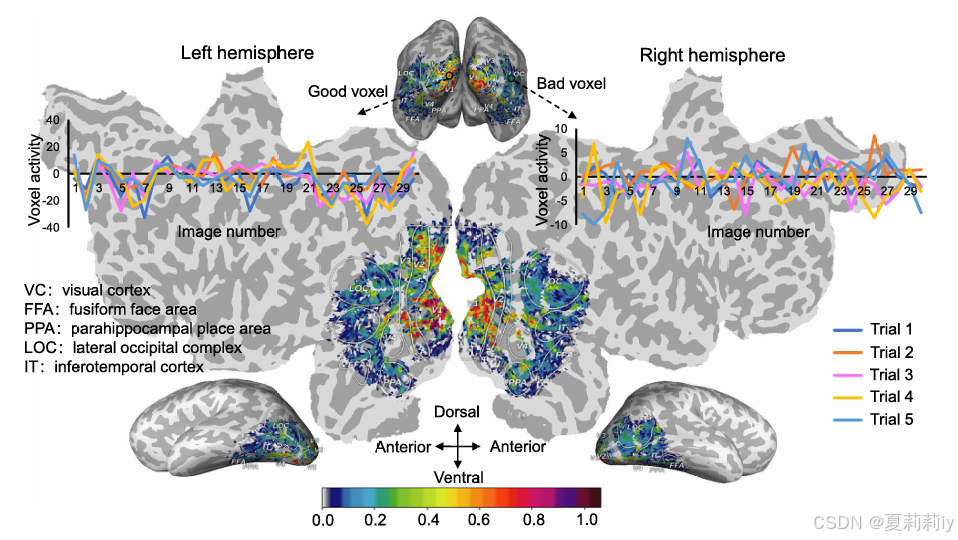
②⭐“为了提高神经解码的稳定性，作者对 fMRI 数据使用了稳定性选择（Pearson），其中选择了在相同视觉刺激的不同试验中激活模式具有最高一致性的体素进行分析”

③Decrease the dimension by discarding unstabled voxels in all the ROIs

④Normalize fMRI data

⑤Applying PCA on fMRI data and doing test

⑥Extracting feature from images by pre trained RepVGG, and futher flatten and normalize data, then apply PCA

⑦Encode text by ALBERT and GPT-Neo, and get sentence embedding by average of token embeddings. “由于 ALBERT 和 GPT-Neo 的输入序列长度受到限制，不能直接将整个 Wikipedia 文章输入到模型中。为了对可以超过最大长度的文章进行编码，也可以将文章文本拆分为部分重叠的 256 个标记序列，其中重叠 50 个标记。连接多个句子嵌入将导致不希望的“维度诅咒”问题。因此，我们使用多个序列的平均池化表示来编码整篇文章。这种平均池化策略也已成功用于最近的语言神经编码研究。同样，如果一个类在 Wikipedia 中有多个对应的文章，我们将对从每个文章中获得的表示进行平均。有关平均池化下文本特征的异质性程度，请参阅附录。”

文章分割成重叠序列例子：假设有一篇包含 1000 tokens 的文章。将其分割成以下几个重叠的序列：

第一段：从第 1 到第 256 个 token（共 256 个 token）

第二段：从第 207 到第 462 个 token（共 256 个 token，与第一段有 50 个 token 的重叠）

第三段：从第 413 到第 668 个 token（共 256 个 token，和第二段有 50 个 token 的重叠）

依此类推。

这样，虽然每个片段的长度为 256 个 token，但它们之间有 50 个 token 重叠，这样模型可以理解不同片段之间的联系和上下文。

平均池化例子：假设有3个片段，它们分别通过模型得到了以下嵌入向量：

第一段的嵌入向量：0.1,0.2,0.3

第二段的嵌入向量：0.2,0.3,0.4

第三段的嵌入向量：0.3,0.4,0.5

将这些向量进行平均池化：

平均向量 = $\frac{1}{3}\times([0.1,0.2,0.3]+[0.2,0.3,0.4]+[0.3,0.4,0.5])$

结果是：

平均向量 = $\left[\frac{0.1+0.2+0.3}{3},\frac{0.2+0.3+0.4}{3},\frac{0.3+0.4+0.5}{3}\right]=[0.2,0.3,0.4]$

类似多篇文章取平均

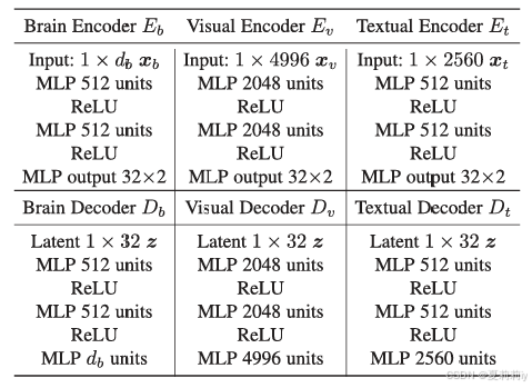
2.4.3. High-Level Overview of the Proposed BraVL Model

①Overall framework of BraVL:

where MoPoE is Mixture-of-Products-of-Experts

2.4.4. Multi-Modality Joint Modeling

①Marginal log-likelihood for single modality $z$ :

$\log p_\theta(\boldsymbol{x})=\log\int p_\theta(\boldsymbol{x}|\boldsymbol{z})p(\boldsymbol{z})d\boldsymbol{z}$

②Due to the difficult of calculating $\log p_\theta(\boldsymbol{x})$ , variational auto-encoders (VAEs) chose to optimize Evidence Lower BOund (ELBO):

$\begin{aligned} \log p_{\theta}(\boldsymbol{x}) & \geq\mathbb{E}_{q_\phi(\boldsymbol{z}|\boldsymbol{x})}[\log p_\theta(\boldsymbol{x}|\boldsymbol{z})]-D_{KL}\left[q_\phi(\boldsymbol{z}|\boldsymbol{x})\|p(\boldsymbol{z})\right] \\ & =\operatorname{ELBO}(\boldsymbol{x}), \end{aligned}$

where $q_\phi(z|\boldsymbol{x})$ denotes approximate posterior distribution represented, $p_\theta(\boldsymbol{z}|\boldsymbol{x})$ is decoder network

③A multimodality ELBO:

$\begin{aligned} \log p_{\Theta}(\mathbb{X})\geq & \mathbb{E}_{q_{\Phi}(\boldsymbol{z}|\mathbb{X})}\bigg[\sum_{\boldsymbol{x}_{m}\in\mathbb{X}}\log p_{\theta_{m}}\left(\boldsymbol{x}_{m}|\boldsymbol{z}\right)\bigg] \\ &-D_{KL}\left[q_\Phi(\boldsymbol{z}|\mathbb{X})\|p(\boldsymbol{z})\right] \\ =& \mathrm{ELBO}(\mathbb{X})\triangleq\mathcal{L}_{M}(\Theta,\Phi), \end{aligned}$

where $p_{\theta_m}(\boldsymbol{x}_m|\boldsymbol{z})$ denotes decoders with multi parameters and modalities $\Theta=\{\theta_m\},m\in\{b,v,t\}$ . seen $\mathbb{X}=\{\boldsymbol{x}_b,\boldsymbol{x}_v,\boldsymbol{x}_t\}$ and unseen $\mathbb{X}=\{\boldsymbol{x}_v,\boldsymbol{x}_t\}$ , $\mathbb{X}_s$ denotes a possible subset of $\mathbb{X}$ , $\mathcal{P}(\mathbb{X})$ denotes all $\mathbb{X}$ subsets

④Optimization methods:

⑤Parameterized $q_\Phi(\boldsymbol{z}|\mathbb{X})$ will be easilyd faced with posterior collapse: a) the joint latent variable $\boldsymbol{z}$ is independent from the observed data $\mathbb{X}$ , b) the decoder may no longer focus on latent variables $\boldsymbol{z}$ , c) lack of consistency between jointly generated modalities

⑥By MoPoE, the loss can be writen as:

$\mathcal{L}_M(\Theta,\Phi)=\mathbb{E}_{q_\Phi(\boldsymbol{z}|\mathbb{X})}\left[\sum_{\boldsymbol{x}_m\in\mathbb{X}}\log p_{\theta_m}\left(\boldsymbol{x}_m|\boldsymbol{z}\right)\right]-D_{KL}\left[\frac{1}{|\mathcal{P}(\mathbb{X})|}\sum_{\mathbb{X}_s\in\mathcal{P}(\mathbb{X})}\prod_{\boldsymbol{x}_m\in\mathbb{X}_s}\times q_{\phi_m}\left(z|x_m\right)\|p(z)\right]$

2.4.5. Mutual Information (MI) Regularization

（1）Intra-Modality MI Maximization

①Variational lower bound on MI between samples of the posterior distribution of joint latent variable $\boldsymbol{z}$ and observation $\boldsymbol{x}_m$ :

$\begin{aligned} & I(\boldsymbol{z};\boldsymbol{x}_{m}) \\ & =H(\boldsymbol{z})-H(\boldsymbol{z}|\boldsymbol{x}_m) \\ & =\mathbb{E}_{\boldsymbol{x}_m\sim p_{\theta_m}(\boldsymbol{x}_m|\boldsymbol{z})}\left[\mathbb{E}_{\boldsymbol{z}\sim q_\Phi(\boldsymbol{z}|\mathbb{X})}[\log p(\boldsymbol{z}|\boldsymbol{x}_m)]\right]+H(\boldsymbol{z}) \\ & =\mathbb{E}_{\boldsymbol{x}_m\sim p_{\theta_m}(\boldsymbol{x}_m|\boldsymbol{z})}[\underbrace{D_{KL}(p(\cdot|\boldsymbol{x}_m)\|Q_{\psi_m}(\cdot|\boldsymbol{x}_m))}_{\geq0} \\ & +\mathbb{E}_{\boldsymbol{z}\sim q_\Phi(\boldsymbol{z}|\mathbb{X})}\left[\log Q_{\psi_m}\left(\boldsymbol{z}|\boldsymbol{x}_m\right)\right]\Big]+H(\boldsymbol{z}) \\ & \geq\mathbb{E}_{\boldsymbol{x}_{m}\sim p_{\theta_{m}}(\boldsymbol{x}_{m}|\boldsymbol{z})}\left[\mathbb{E}_{\boldsymbol{z}\sim q_{\Phi}(\boldsymbol{z}|\boldsymbol{X})}\left[\log Q_{\psi_{m}}\left(\boldsymbol{z}|\boldsymbol{x}_{m}\right)\right]\right]+H(\boldsymbol{z}) \end{aligned}$

where $Q_{\psi_{m}}$ is some auxiliary distribution implemented by a deepneural network

②Through InfoGAN, they change the bound by:

$\begin{aligned} I(\boldsymbol{z};\boldsymbol{x}_{m}) & \geq\mathbb{E}_{\boldsymbol{z}\sim q_{\Phi}(\boldsymbol{z}|\mathbb{X}),\boldsymbol{x}_{m}\sim p_{\theta m}(\boldsymbol{x}_{m}|\boldsymbol{z})} \\ & \times[\log Q_{\psi_{m}}(\boldsymbol{z}|\boldsymbol{x}_{m})]+H(\boldsymbol{z}) \end{aligned}$

③There is $\mathbb{E}_{x\sim X,y\sim Y|x}[f(x,y)]=\mathbb{E}_{x\sim X,y\sim Y|x,x^{\prime}\sim X|y}[f(x^{\prime},y)]$

④Intra loss:

$\begin{aligned} \mathcal{L}_{intra}(\Theta,\Phi,\Psi) & =\sum_{m}\mathbb{E}_{\boldsymbol{z}\sim q_{\Phi}(\boldsymbol{z}|\mathbb{X}),\boldsymbol{x}_{m}\sim p_{\theta m}(\boldsymbol{x}_{m}|\boldsymbol{z})} \\ & \times[\log Q_{\psi_{m}}\left(\boldsymbol{z}|\boldsymbol{x}_{m}\right)]+H(\boldsymbol{z}) \end{aligned}$

（2）Inter-Modality MI Maximization

①The seen inter modality loss:

$\mathcal{L}_{inter}(\Theta,\Phi)\\=I\left(\boldsymbol{x}_b,\boldsymbol{x}_v;\boldsymbol{x}_t\right)+I\left(\boldsymbol{x}_b;\boldsymbol{x}_v,\boldsymbol{x}_t\right)+I\left(\boldsymbol{x}_b,\boldsymbol{x}_t;\boldsymbol{x}_v\right)\\ =\log\frac{P_{\Theta}\left(\boldsymbol{x}_{b},\boldsymbol{x}_{v},\boldsymbol{x}_{t}\right)}{P_{\Theta}\left(\boldsymbol{x}_{b},\boldsymbol{x}_{v}\right)p_{\Theta}\left(\boldsymbol{x}_{t}\right)}+\log\frac{P_{\Theta}\left(\boldsymbol{x}_{b},\boldsymbol{x}_{v},\boldsymbol{x}_{t}\right)}{P_{\Theta}\left(\boldsymbol{x}_{b}\right)p_{\Theta}\left(\boldsymbol{x}_{v},\boldsymbol{x}_{t}\right)}+\log\frac{P_{\Theta}\left(\boldsymbol{x}_{b},\boldsymbol{x}_{v},\boldsymbol{x}_{t}\right)}{P_{\Theta}\left(\boldsymbol{x}_{b},\boldsymbol{x}_{t}\right)p_{\Theta}\left(\boldsymbol{x}_{v}\right)}\\ \approx\log\frac{P_{\Theta}\left(\boldsymbol{x}_{b},\boldsymbol{x}_{v},\boldsymbol{x}_{t}\right)}{\sum_{\boldsymbol{x}_{t}^{\prime}}P_{\Theta}\left(\boldsymbol{x}_{b},\boldsymbol{x}_{v},\boldsymbol{x}_{t}^{\prime}\right)\sum_{\boldsymbol{x}_{b}^{\prime}}\sum_{\boldsymbol{x}_{v}^{\prime}}P_{\Theta}\left(\boldsymbol{x}_{b}^{\prime},\boldsymbol{x}_{v}^{\prime},\boldsymbol{x}_{t}\right)}\\ +\log\frac{P_{\Theta}\left(\boldsymbol{x}_{b},\boldsymbol{x}_{v},\boldsymbol{x}_{t}\right)}{\sum_{\boldsymbol{x}_{v}^{\prime}}\sum_{\boldsymbol{x}_{t}^{\prime}}P_{\Theta}\left(\boldsymbol{x}_{b},\boldsymbol{x}_{v}^{\prime},\boldsymbol{x}_{t}^{\prime}\right)\sum_{\boldsymbol{x}_{b}^{\prime}}P_{\Theta}\left(\boldsymbol{x}_{b}^{\prime},\boldsymbol{x}_{v},\boldsymbol{x}_{t}\right)}\\ +\log\frac{P_{\Theta}\left(x_{b},x_{v},x_{t}\right)}{\sum_{x_{v}^{\prime}}P_{\Theta}\left(x_{b},x_{v}^{\prime},x_{t}\right)\sum_{x_{b}^{\prime}}\sum_{x_{t}^{\prime}}P_{\Theta}\left(x_{b}^{\prime},x_{v},x_{t}^{\prime}\right)}\\ =3\log P_{\Theta}\underbrace{(\boldsymbol{x}_{b},\boldsymbol{x}_{v},\boldsymbol{x}_{t})}_{positive}-\log\sum_{\boldsymbol{x}_{t}^{^{\prime}}}P_{\Theta}\underbrace{(\boldsymbol{x}_{b},\boldsymbol{x}_{v},\boldsymbol{x}_{t}^{^{\prime}})}_{negative}\\ -\log\sum_{x_{b}^{^{\prime}}}\sum_{x_{v}^{^{\prime}}}P_{\Theta}\underbrace{(\boldsymbol{x}_{b}^{\prime},\boldsymbol{x}_{v}^{\prime},\boldsymbol{x}_{t})}_{negative}-\log\sum_{\boldsymbol{x}_{v}^{^{\prime}}}\sum_{\boldsymbol{x}_{t}^{^{\prime}}}P_{\Theta}\underbrace{(\boldsymbol{x}_{b},\boldsymbol{x}_{v}^{\prime},\boldsymbol{x}_{t}^{\prime})}_{negative}\\ -\log\sum_{x_{b}^{^{\prime}}}P_{\Theta}\underbrace{(\boldsymbol{x}_{b}^{^{\prime}},\boldsymbol{x}_{v},\boldsymbol{x}_{t})}_{negative}-\log\sum_{x_{v}^{^{\prime}}}P_{\Theta}\underbrace{(\boldsymbol{x}_{b},\boldsymbol{x}_{v}^{^{\prime}},\boldsymbol{x}_{t})}_{negative}\\ -\log\sum_{x_{b}^{^{\prime}}}\sum_{x_{t}^{^{\prime}}}P_{\Theta}\underbrace{(\boldsymbol{x}_{b}^{\prime},\boldsymbol{x}_{v},\boldsymbol{x}_{t}^{\prime})}_{negative}$

②They add a χ-upper-bound(CUBO) estimator to limite the upper bound:

$\begin{aligned} \mathrm{ELBO} & \leq\log p_{\Theta}(\mathbb{X}) \\ & \leq\underbrace{\mathbb{E}_{\left\{\boldsymbol{z}_{k}\right\}_{1}^{K}\sim q_{\Phi}}\left[\log\sqrt[2]{\frac{1}{K}\sum_{k=1}^{K}\left(\frac{p_{\Theta}\left(\boldsymbol{z}_{k},\mathbb{X}\right)}{q_{\Phi}\left(\boldsymbol{z}_{k}|\mathbb{X}\right)}\right)^{2}}\right]}_{\mathrm{CUBO}} \end{aligned}$

③Inter loss for novel class:

$\begin{aligned} & \mathcal{L}_{inter}(\Theta,\Phi)=I(\boldsymbol{x}_{v};\boldsymbol{x}_{t}) \\ & =\log\frac{P_{\Theta}\left(x_{v},x_{t}\right)}{P_{\Theta}\left(x_{v}\right)p_{\Theta}\left(x_{t}\right)} \\ & \approx\log\frac{P_{\Theta}\left(\boldsymbol{x}_{v},\boldsymbol{x}_{t}\right)}{\sum_{\boldsymbol{x}_{t}^{\prime}}P_{\Theta}\left(\boldsymbol{x}_{v},\boldsymbol{x}_{t}^{\prime}\right)\sum_{\boldsymbol{x}_{v}^{\prime}}P_{\Theta}\left(\boldsymbol{x}_{v}^{\prime},\boldsymbol{x}_{t}\right)} \\ & =\log P_{\Theta}\underbrace{(\boldsymbol{x}_{v},\boldsymbol{x}_{t})}_{positive}-\log\sum_{\boldsymbol{x}_{t}^{\prime}}P_{\Theta}\underbrace{(\boldsymbol{x}_{v},\boldsymbol{x}_{t}^{\prime})}_{negative}-\log\sum_{\boldsymbol{x}_{v}^{\prime}}P_{\Theta}\underbrace{(\boldsymbol{x}_{v}^{\prime},\boldsymbol{x}_{t})}_{negative}, \end{aligned}$

2.4.6. Overall Objective and Training

①Total loss:

$\max_{\Theta,\Phi}\max_{\Psi}\mathcal{L}(\Theta,\Phi,\Psi)=\mathcal{L}_{M}(\Theta,\Phi)+\lambda_{1}\mathcal{L}_{intra}(\Theta,\Phi,\Psi)+\lambda_2\mathcal{L}_{inter}(\Theta,\Phi)$

②Training process:

③Classifier: SVM

2.5. Experiments

2.5.1. Brain-Visual-Linguistic Datasets

①Statistcs of datasets:

②Used EEG signals:

2.5.2. Implementation Detail

①Parameters:

②Stability of ROIs:

2.5.3. Results

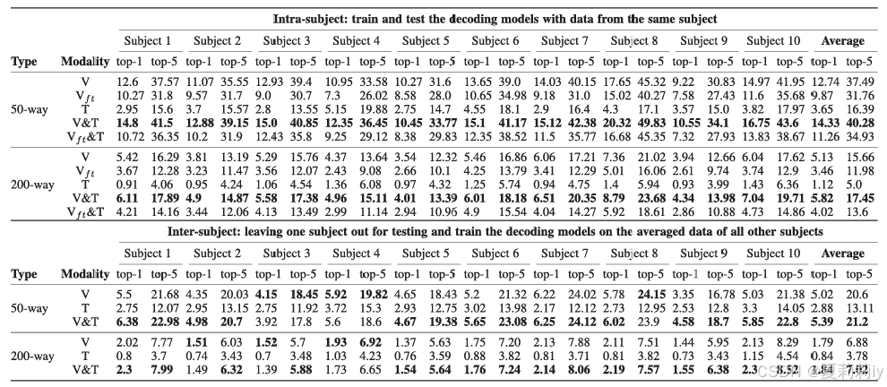
（1）Does Language Influence Vision?

①Performance table:

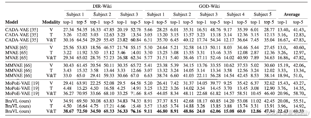
②The benefits brought by text assisted training:

③The impact of text prompts on brain regions:

（2）Are Wiki Articles More Effective Than Class Names?

①Decoder ablation:

（3）Ablation Study

①Loss ablation:

②Joint posterior approximation ablation:

（4）Sensitivity Analysis

①Hyperparameters ablation:

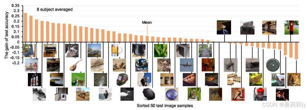
（5）Analyzing the Impact of Extra Data

①Benefits from extra data:

（6）Cross-Modality Generation for Brain Activity

①t-SNE of real (blue) and generated (orange) images:

（7）Performance of Different Brain Areas

①ROI ablation:

②Importance of ROIs:

（8）Evaluation on the ThingsEEG-Text Dataset

①Performance on ThingsEEG-Text dataset:

（9）Fine-Tuning the Feature Extractors

①No need

2.6. Discussion

2.7. Conclusion

3. 知识补充

3.1. Product-of-experts formulation

（1）参考学习：Product-of-Experts（PoE） - 知乎

4. Reference

Du, C. et al. (2023) Decoding Visual Neural Representations by Multimodal Learning of Brain-Visual-Linguistic Features, IEEE Transactions on Pattern Analysis and Machine Intelligence, 45(9): 10760-10777. doi: 10.1109/TPAMI.2023.3263181