机器学习_手写算法：Adaboost简单实现

Adaboost 是基于错误率迭代，增加错误分类的权重，加重优分类器的权重。

---

统计学习方法Adaboost例题

假设分类器有 x <v 或者 x>v产生，其阈值v使该分类器在训练集上分类误差最低。试用Adaboost算法学习一个强分类器

1、首先观察数据（由于是二维的可以直接画图）

import  matplotlib.pyplot as plt
plt.style.use('ggplot') 
x = np.array(list(range(10)))
y = np.array([1, 1, 1, -1, -1, -1, 1, 1, 1, -1])
# 图示
plt.scatter(x,y)
plt.show()

2、定义分类器

# 基分类器
def h(x, v, b):
    return (x < v) * -1*b + (x > v) * b

3、计算错误率

错误率为错误的样本的权重之和

# 基于错误率优化分类器
def find_error(x, v, b):
	# 找到错误的样本位置
    return np.where(x == x)[0][[h(x, v, b) != y]]
# 错误率为错误的样本的权重之和
e = sum(w[find_error(x, v, b)])     

4、根据错误率找到当前最佳分类器

def find_v(x, w):
    z1,z2 , out1, out2 = 1, 1, 0,0
    for v in (x+0.5):
        a1 = sum(w[find_error(x, v, 1)])
        if z1 > a1:  # 寻找全局最低错误率
            z1, out1 = a1, v
    for v in (x+0.5):
        a2 = sum(w[find_error(x, v, -1)])
        if z2 > a2:  # 寻找全局最低错误率
            z2, out2 = a2, v
    if z1 < z2:
        return out1, 1
    else:
        return out2, -1

5、Adaboost算法

def Adaboost_t(x, y, w_):
    # 返回最终分类器公式
    w = w_
    div = 0
    message = ''
    while sum(div != y):
        v , b = find_v(x, w)
        e = sum(w[find_error(x, v, b)])
        ## 基分类器权重
        alpha = 0.5* np.log((1 - e)/ e)  # 加大优的分类器的权重
        ## 样本权重损失函数
        w_loss = np.array([np.exp(-1 *alpha * y[i] * h(x[i], v, b)) for i in range(len(x))])  #  加大错误样本的关注度
        ## 计算常数
        Z = sum(w_loss * w)
        # 分布变化
        w = w * w_loss / Z
        div += h(x, v, b)  #分类器迭代
        message += 'h(x, '+str(v) +','+str(b) +')' +'*' +str(alpha) + "+"
    return ('G(x)' + "=" + message)[:-1]

def Adaboost_sign(x, a):
    # 将分类器公式转换成可执行
    # a 为文本公式
    import re
    hx_all = re.findall(r'h\(.*?\)',a)
    alpha_all = re.findall(r'\*0.\d*', a)
    n = len(hx_all)
    out = 0
    v,b=0,0
    for i in range(n):
        alpha = np.float(alpha_all[i][1:])
        v = np.float(hx_all[i].replace(')','').split(',')[1])
        b = np.float(hx_all[i].replace(')','').split(',')[-1])
        out += alpha*h(x, v, b)
    return np.sign(out)

最终运算

w_1 = np.array([1]).repeat(10)/10
a = Adaboost_t(x, y, w_1)  
# 结果 ==> >  'G(x)=h(x, 2.5,-1)*0.4236489301936017+h(x, 8.5,-1)*0.6496414920651304+h(x, 5.5,1)*0.752038698388137'
Adaboost_sign(x, a)  #  array([ 1.,  1.,  1., -1., -1., -1.,  1.,  1.,  1., -1.])

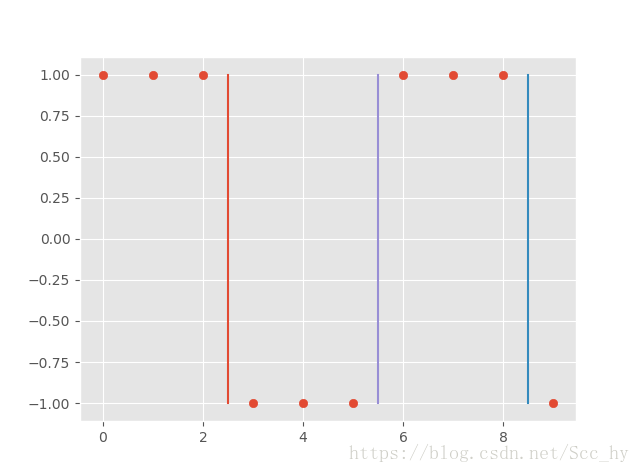
图示最终分类器

# 图示
plt.scatter(x,y)
plt.plot([2.5,2.5],[-1,1])
plt.plot([8.5,8.5],[-1,1])
plt.plot([5.5,5.5],[-1,1])
plt.show()

Adaboost的基分类器可采用不同的弱分类器，该习题仅仅用了最简单的垂线分类器。
目前该脚本的实用性有限，仅作为练习和娱乐，后期笔者会进行优化。