机器学习-Receiver Operating Charateristic(ROC)

Section I: Brief Introduction on ROC Curve

Receiver Operating Charateristic(ROC) graphs are usefult tools to select models forclassification based on their performance with respect to th FPR and TPR, which are computed by shifting the decision threshold of the classifier. The diagonal of an ROC graph can be interpreted as random guessing, and classification models that fall below the diagonal are considered as worse than random guessing. A perfect classifier would fall into the top left corner of the graph with a TPR of 1 and an FOR of 0. Then, ROC area under the curve (ROC AUC) to charaterize the classification performance can be subsequently computed.

FROM
Sebastian Raschka, Vahid Mirjalili. Python机器学习第二版. 南京：东南大学出版社，2018.

Section II: Code Bundle and Result Analyses

第一部分：代码：

from sklearn import datasets
from sklearn.model_selection import train_test_split
from sklearn.preprocessing import StandardScaler
from sklearn.linear_model import LogisticRegression
from sklearn.decomposition import PCA
from sklearn.pipeline import make_pipeline
from sklearn.model_selection import StratifiedKFold
from sklearn.metrics import roc_curve,auc
import numpy as np
from scipy import interp
import matplotlib.pyplot as plt
import warnings
warnings.filterwarnings("ignore")

plt.rcParams['figure.dpi']=200
plt.rcParams['savefig.dpi']=200
font = {'family': 'Times New Roman',
        'weight': 'light'}
plt.rc("font", **font)

#Section 1: Load Breast data, i.e., Benign and Malignant
breast=datasets.load_breast_cancer()
X=breast.data
y=breast.target
X_train,X_test,y_train,y_test=\
    train_test_split(X,y,test_size=0.2,stratify=y,random_state=1)

#Section 2: Construct model optimized via GridSearch
pipe_lr=make_pipeline(StandardScaler(),\
                      PCA(n_components=2),\
                      LogisticRegression(penalty='l2',random_state=1,C=100))

cv=list(StratifiedKFold(n_splits=3,random_state=1).split(X_train,y_train))
fig=plt.figure(figsize=(7,5))
mean_tpr=0
mean_fpr=np.linspace(0,1,100)
all_tpr=[]

for i,(train_idx,test_idx) in enumerate(cv):
    probas=pipe_lr.fit(X_train[train_idx],y_train[train_idx]).predict_proba(X_train[test_idx])
    fpr,tpr,thresholds=roc_curve(y_train[test_idx],probas[:,1],pos_label=1)
    mean_tpr+=interp(mean_fpr,fpr,tpr)
    mean_tpr[0]=0
    roc_auc=auc(fpr,tpr)
    plt.plot(fpr,
             tpr,
             label='ROC Fold %d (Area = %.2f)' % (i+1,roc_auc))

plt.plot([0,1],[0,1],linestyle='--',color=[0.6,0.6,0.6],label='Random Guessing')
mean_tpr/=len(cv)
mean_tpr[-1]=1.0
mean_auc=auc(mean_fpr,mean_tpr)
plt.plot(mean_fpr,
         mean_tpr,
         'k--',
         label="Mean ROC (Area = %0.2f)" % mean_auc,
         linewidth=2)
plt.plot([0,0,1],[0,1,1],linestyle=":",color='black',label='Perfect Performance')
plt.xlim([-0.05,1.05])
plt.ylim([-0.05,1.05])
plt.xlabel("False Positive Rate")
plt.ylabel("True Positive Rate")
plt.legend(loc='lower right')
plt.savefig('./fig1.png')
plt.show()

第二部分：结果：

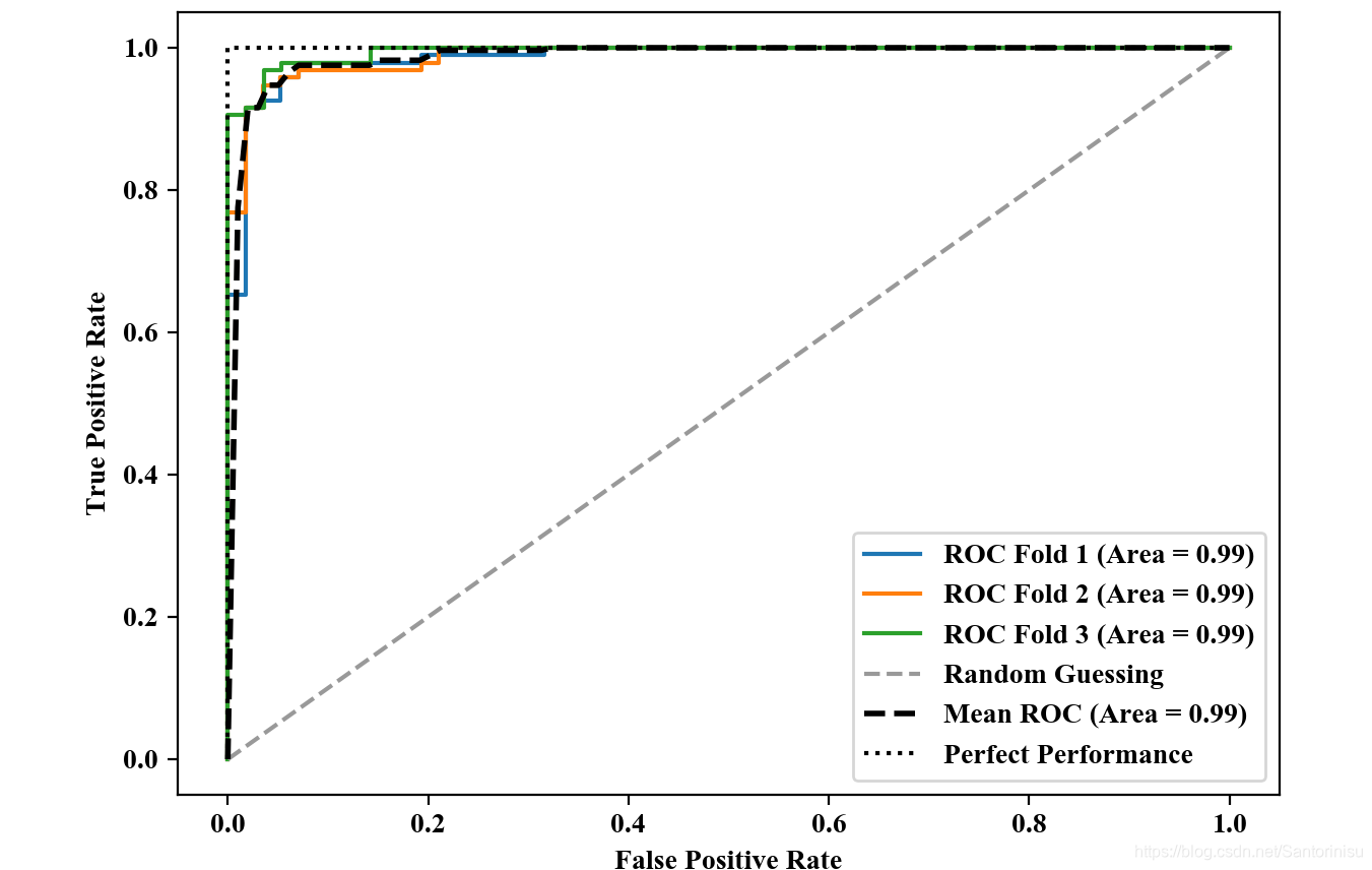
值得注意，曲线下方面积越大，FPR越小，说明负类辨识精准，TPR越高说明正类辨识越准确。由此可进一步说明模型分类性能越佳。

参考文献：
Sebastian Raschka, Vahid Mirjalili. Python机器学习第二版. 南京：东南大学出版社，2018.