Technical Blog: Sentiment Analysis of IMDB Movie Reviews

原创已于 2024-12-14 17:19:32 修改 · 829 阅读

CC 4.0 BY-SA版权

文章标签：

于 2024-12-12 15:44:25 首次发布

In blog 1 I importing necessary packages, loading data, and data preprocessing. My blog2 is expected to include feature extraction, model training, model evaluation, visualization, and conclusions.

Step 1. Import packages

Step 2. Import the training data and data pre-processing

You could check my blog 1 here:

Technical Blog: Sentiment Analysis of IMDB Movie Reviews-优快云博客

In Blog 2, I would introduce the left steps which are feature extraction, model training, model evaluation, visualization, and conclusion.

Step 3. Feature Extraction

This section focuses on transforming raw data into a structured format suitable for analysis. Feature extraction involves selecting and engineering attributes that will be input to the model, which directly impacts its performance. Techniques may include vectorization, dimensionality reduction, or encoding categorical variables.

In this section, I will introduce some methods to accomplish feature extraction:

1). BOW
2). TF-IDF
3). Label Encoding
4). Train-Test Split

1). BOW

#Bags of words model

#Count vectorizer for bag of words
cv=CountVectorizer(min_df=1,max_df=1.0,binary=False,ngram_range=(1,3))
#transformed train reviews
cv_train_reviews=cv.fit_transform(norm_train_reviews)
#transformed test reviews
cv_test_reviews=cv.transform(norm_test_reviews)

print('BOW_cv_train:',cv_train_reviews.shape)
print('BOW_cv_test:',cv_test_reviews.shape)
#vocab=cv.get_feature_names()-toget feature names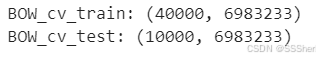

BOW_cv_train: Training data contains 40,000 comments. There are 6,983,233 different n-gram features.

BOW_cv_test: Testing data contained 10,000 comments. The feature space of the test data was consistent with the training data, still 6,983,233 features.

2). TF-IDF

#TF-IDF
tv=TfidfVectorizer(min_df=1,max_df=1.0,use_idf=True,ngram_range=(1,3))
#transformed train reviews
tv_train_reviews=tv.fit_transform(norm_train_reviews)
#transformed test reviews
tv_test_reviews=tv.transform(norm_test_reviews)
print('Tfidf_train:',tv_train_reviews.shape)
print('Tfidf_test:',tv_test_reviews.shape)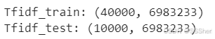

Tfidf_train: 40000 training comments, 6983233 unique n-gram features extracted from the data.

Tfidf_test:(1000 testing comments0,6983233 unique n-gram features extracted from the data as the training data.

3). Label Encoding

#Labeling the sentiment data
lb = LabelBinarizer()

#Transformed sentiment data
sentiment_data = lb.fit_transform(imdb_data['sentiment'])
print(sentiment_data.shape)

There were 50,000 samples in the dataset, and each sample corresponds to a binary label.

4). Train-Test Split

#Split the sentiment data
train_sentiments = sentiment_data[:40000]
test_sentiments = sentiment_data[40000:]
print(train_sentiments)
print(test_sentiments)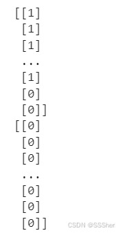

The first 40,000 samples were used for model training. The latter 10,000 samples were used for model testing.

1 Indicates positive feelings (Positive). 0 Indicates negative feelings (Negative)

Step 4. Model Training

# Logistic Regression model
lr = LogisticRegression(penalty='l2', max_iter=500, C=1, random_state=42)

# Reshape target variable (y_train)
y_train = train_sentiments.ravel()

# Fit the model for Bag of Words features
lr_bow = lr.fit(cv_train_reviews, y_train)
print(lr_bow)

# Fit the model for TF-IDF features
lr_tfidf = lr.fit(tv_train_reviews, y_train)
print(lr_tfidf)

Models trained with Bag of Words features and TF-IDF features.

The output shows that both models use the same hyperparameters and complete the training successfully.

#make sure it is numpy.ndarray

print(type(train_sentiments))
print(train_sentiments.shape)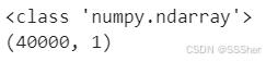

#check the null values

print("Shape of train_sentiments:", train_sentiments.shape)
print("Any NaN values:", np.isnan(train_sentiments).any())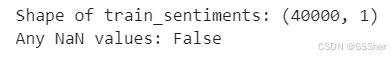

Step 5. Model Evaluation

In this section, I will introduce some methods to accomplish model evaluation:

1). Logistic Regression
2). confusion matrix
3). SGDClassifier
4). Multinomial Naive Bayes (MNB)

1). Logistic Regression

A binary classification model based on Logistic Regression was trained and its performance was evaluated.


from sklearn.linear_model import LogisticRegression
from sklearn.preprocessing import LabelEncoder
from sklearn.metrics import accuracy_score, classification_report

# Encode the target variable numerical values
le = LabelEncoder()
train_sentiments_encoded = le.fit_transform(train_sentiments.ravel())  # Coding of train_sentiments
test_sentiments_encoded = le.transform(test_sentiments.ravel())        # Coding of test_sentiments

# Check the shape
print('train_sentiments_encoded shape:', train_sentiments_encoded.shape)  # (40000,)
print('test_sentiments_encoded shape:', test_sentiments_encoded.shape)    #  (10000,)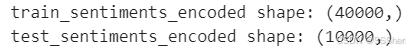

#Logistic regression model performance on test dataset

#Predict the model for bag of words
lr_bow_predict=lr.predict(cv_test_reviews)
print(lr_bow_predict)

#Predict the model for tfidf features
lr_tfidf_predict=lr.predict(tv_test_reviews)
print(lr_tfidf_predict)

#Accuracy of the models
#Accuracy score for bag of words
lr_bow_score=accuracy_score(test_sentiments_encoded,lr_bow_predict)
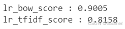
print("lr_bow_score :",lr_bow_score)

#Accuracy score for tfidf features
lr_tfidf_score=accuracy_score(test_sentiments_encoded,lr_tfidf_predict)
print("lr_tfidf_score :",lr_tfidf_score)

#Print the classification report
#Classification report for bag of words 
lr_bow_report=classification_report(test_sentiments_encoded,lr_bow_predict,target_names=['Positive','Negative'])
print(lr_bow_report)

#Classification report for tfidf features
lr_tfidf_report=classification_report(test_sentiments_encoded,lr_tfidf_predict,target_names=['Positive','Negative'])
print(lr_tfidf_report)

Accuracy: the accuracy of the model on the test set (the proportion of correct predictions).

Precision: the proportion of positive classes predicted correctly.

Recall: the percentage of actual positive classes that are correctly predicted.

F1-score: a balanced average of accuracy and recall.

Support: number of samples in each class.

2). Confusion Matrix

The confusion matrix of the model based on Bag of Words and TF-IDF features on the test set is calculated.

#Confusion matrix
#confusion matrix for bag of words
cm_bow=confusion_matrix(test_sentiments_encoded,lr_bow_predict,labels=[1,0])
print(cm_bow)

#confusion matrix for tfidf features
cm_tfidf=confusion_matrix(test_sentiments_encoded,lr_tfidf_predict,labels=[1,0])
print(cm_tfidf)

General interpretation of the output:
[[TP, FN],
[FP, TN]]

TP (True Positive): actual is positive class, predicted is positive class.
FN (False Negative): actual positive class, predicted negative class.
FP (False Positive): actual is negative class, predicted is positive class.
TN (True Negative): Actual is a negative class, predicted is a negative class.

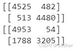
In this case:

BOW:
[[4525 482]
[ 513 4480]]

TP = 4525
FN = 482
FP = 513
TN = 4480 \

TF-IDF:
[[4953 54]
[1788 3205]]

TP =49535
FN =542
FP =17883
TN =32050

3). SGDClassifier

The SGDClassifier of the model based on Bag of Words and TF-IDF features.

#Linear support vector machines for bag of words and tfidf features
#training the linear svm
svm=SGDClassifier(loss='hinge',max_iter=500,random_state=42)

#fitting the svm for bag of words
svm_bow=svm.fit(cv_train_reviews,train_sentiments_encoded)
print(svm_bow)

#fitting the svm for tfidf features
svm_tfidf=svm.fit(tv_train_reviews,train_sentiments_encoded)
print(svm_tfidf)

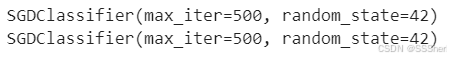
The output shows that both models have been successfully trained.
Configure the display to show the maximum number of iterations 'max_iter=500' and the random seed 'random_state=42'.

#Model performance on test data
#Predicting the model for bag of words
svm_bow_predict=svm.predict(cv_test_reviews)
print(svm_bow_predict)

#Predicting the model for tfidf features
svm_tfidf_predict=svm.predict(tv_test_reviews)
print(svm_tfidf_predict)

#Accuracy of the model
#Accuracy score for bag of words
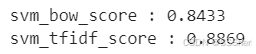
svm_bow_score=accuracy_score(test_sentiments_encoded,svm_bow_predict)
print("svm_bow_score :",svm_bow_score)

#Accuracy score for tfidf features
svm_tfidf_score=accuracy_score(test_sentiments_encoded,svm_tfidf_predict)
print("svm_tfidf_score :",svm_tfidf_score)

#Print the classification report
#Classification report for bag of words 
svm_bow_report=classification_report(test_sentiments_encoded,svm_bow_predict,target_names=['Positive','Negative'])
print(svm_bow_report)

#Classification report for tfidf features
svm_tfidf_report=classification_report(test_sentiments_encoded,svm_tfidf_predict,target_names=['Positive','Negative'])
print(svm_tfidf_report)

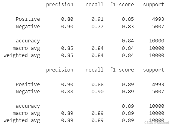
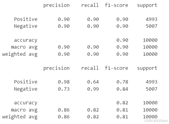
BOW(up):
Positive Class (Positive Sentiment):
Precision: 80% of predicted positive sentiments were correct.
Recall: 91% of actual positive sentiments were correctly identified.
F1-score: 85%, reflecting a balance between precision and recall. \

Negative Class (Negative Sentiment):
Precision: 90% of predicted negative sentiments were correct.
Recall: 77% of actual negative sentiments were correctly identified.
F1-score: 83%.

Overall Performance:
Accuracy: 84%.
Macro Average: 84% (average performance across both classes).
Weighted Average: 84% (weighted by the number of samples in each class).

TF-IDF(down):
Positive Class (Positive Sentiment):
Precision: 90% of predicted positive sentiments were correct.
Recall: 88% of actual positive sentiments were correctly identified.
F1-score: 89%.

Negative Class (Negative Sentiment):
Precision: 88% of predicted negative sentiments were correct.
Recall: 89% of actual negative sentiments were correctly identified.
F1-score: 89%.

Overall Performance:
Accuracy: 89%.
Macro Average: 89%.
Weighted Average: 89%.

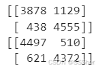
#Plot the confusion matrix
#confusion matrix for bag of words
cm_bow=confusion_matrix(test_sentiments_encoded,svm_bow_predict,labels=[1,0])
print(cm_bow)

#confusion matrix for tfidf features
cm_tfidf=confusion_matrix(test_sentiments_encoded,svm_tfidf_predict,labels=[1,0])
print(cm_tfidf)

4). Multinomial Naive Bayes Model(MNB)

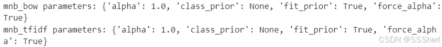
This code trains a Multinomial Naive Bayes (MNB) classifier on Bag of Words and TF-IDF features, and prints the model's hyperparameters.

#Multinomial Naive Bayes for bag of words and tfidf features
#training the model
mnb=MultinomialNB()

#fitting the svm for bag of words
mnb_bow=mnb.fit(cv_train_reviews,train_sentiments_encoded)
print("mnb_bow parameters:", mnb_bow.get_params())

#fitting the svm for tfidf features
mnb_tfidf=mnb.fit(tv_train_reviews,train_sentiments_encoded)
print("mnb_tfidf parameters:", mnb_tfidf.get_params())

from sklearn.metrics import accuracy_score, classification_report

# Prediction and evaluate using the Bag of Words feature
bow_predictions = mnb_bow.predict(cv_test_reviews)
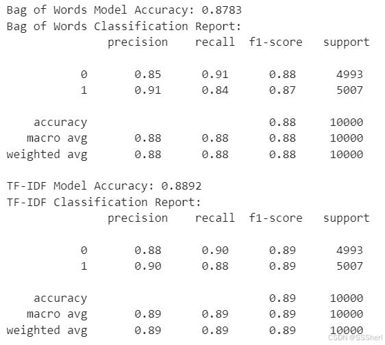
print("Bag of Words Model Accuracy:", accuracy_score(test_sentiments, bow_predictions))
print("Bag of Words Classification Report:\n", classification_report(test_sentiments, bow_predictions))

# Prediction and evaluation of TF-IDF characteristics
tfidf_predictions = mnb_tfidf.predict(tv_test_reviews)
print("TF-IDF Model Accuracy:", accuracy_score(test_sentiments, tfidf_predictions))
print("TF-IDF Classification Report:\n", classification_report(test_sentiments, tfidf_predictions))

#Accuracy of the model
#Accuracy score for bag of words
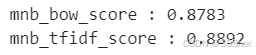
mnb_bow_score=accuracy_score(test_sentiments_encoded,mnb_bow_predict)
print("mnb_bow_score :",mnb_bow_score)

#Accuracy score for tfidf features
mnb_tfidf_score=accuracy_score(test_sentiments_encoded,mnb_tfidf_predict)
print("mnb_tfidf_score :",mnb_tfidf_score)

#Plot the confusion matrix
#confusion matrix for bag of words
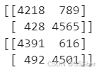
cm_bow=confusion_matrix(test_sentiments_encoded,mnb_bow_predict,labels=[1,0])
print(cm_bow)

#confusion matrix for tfidf features
cm_tfidf=confusion_matrix(test_sentiments_encoded,mnb_tfidf_predict,labels=[1,0])
print(cm_tfidf)

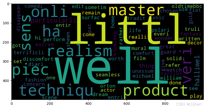
Step 6. Visualization

Plotting word clouds to show the most frequent words in positive and negative comments.

#Word cloud for positive review words
plt.figure(figsize=(10,10))
positive_text=norm_train_reviews[1]
WC=WordCloud(width=1000,height=500,max_words=500,min_font_size=5)
positive_words=WC.generate(positive_text)
plt.imshow(positive_words,interpolation='bilinear')
plt.show

#Word cloud for negative review words
plt.figure(figsize=(10,10))
negative_text=norm_train_reviews[8]
WC=WordCloud(width=1000,height=500,max_words=500,min_font_size=5)
negative_words=WC.generate(negative_text)
plt.imshow(negative_words,interpolation='bilinear')
plt.show