Transformer | 相对位置编码_swin transformer cpb-优快云博客

本文链接：https://blog.youkuaiyun.com/P_LarT/article/details/145248107

Transformer | 相对位置编码

本文作于十月 3日 2022。

过往的相关内容：

在这里插入图片描述

相对位置编码现在已经被很多的视觉 Transformer 使用，也存在不同的实现形式。由于位置编码的本质就是将可学习变量或者是固定参数与特定的位置索引关联起来，所以实现的过程中会涉及到大量的坐标索引的变换，可读性很差。也因此不同形式的实现也存在着明显的差异。

在 NAT 的代码中，注意到了其位置编码的实现不同于之前所见过的形式，于是进行了仔细的分析，并于作者进行了一些讨论。在这个过程中意识到了 NAT 这里的实现形式所具有的的通用性。

本文希望通过对现有代码的分析，以更好的理解相对位置编码的实现的基本策略，尽可能避免未来面对新的实现形式时再次出现困惑。

基本模式

如前所述，位置编码的本质就是将参数与位置相关联。这里的参数指的是一些特定的可学习变量或者是固定的数据。由于现有主流的形式不再使用原始 Transformer 中引入的固定参数的绝对位置编码形式，改为可学习的相对位置编码，所以这里的分析也延续可学习的参数形式。

相对位置编码重点强调一个空间坐标上的相对关系。由于体现的是相对的坐标关系，所以就会存在正负，即位置之间的前后相对关系。相对位置编码多会与窗口的概念相结合。因此相对位置编码非常适合搭配着窗口注意力一起使用。由于需要表示相对位置，所以相对位置编码的参数矩阵 $\mathbf{R}$ 的元素数量一般为 $2W-1)^2$ ，这里 $W$ 表示方形窗口的边长。所以实际上存储相对位置编码的空间也要大于实际的窗口空间（ $\times W$ ）的平方的。

由于不同的位置信息注入的形式会导致位置编码的具体格式有所差异。为了更好的说明问题，这里以常见的 $Q K + E$ 的位置编码组合形式为例进行介绍。

假定 $W = 3$ ，此时的相对位置编码的参数矩阵 $\mathbf{R}$ 的各个位置所实际对应参与 Attention 计算的 Q 和 K 的位置 $q_h,q_w)$ 与 $k_h,k_w)$ 的相对关系 $k_h-q_h,k_w-q_w)$ 分别为：

(-2, -2), (-2, -1), (-2, 0), (-2, 1), (-2, 2), 
(-1, -2), (-1, -1), (-1, 0), (-1, 1), (-1, 2), 
(0, -2), (0, -1), (0, 0), (0, 1), (0, 2),
(1, -2), (1, -1), (1, 0), (1, 1), (1, 2),
(2, -2), (2, -1), (2, 0), (2, 1), (2, 2),

这里的 (-2, -1) 表示，k 位于 q 的左上方。

所以 $Q K + E$ 的运算，也就是将 $\mathbf{R}$ 中的数据，通过特定的索引方式构造成 $E$ ，从而附加 $Q K$ 上有着对应的相对位置关系的位置上。不同的实现中，主要是从 $R$ 到 $E$ 的过程有所差异。

典型工作

典型的工作有 Swin Transformer 和 NAT，这两封工作存在共性，但是 Attention 的具体形式不同。差异主要来自于 qkv 来自的局部邻域的定义。前者是从固定的局部矩形窗口中抽取局部注意力的全部 q、k、v，而后者则将 k、v 的抽取范围定为了 q 为中心的局部邻域，[[…/200-文献笔记/论文记录/4-目标分类/Neighborhood Attention Transformer | 更类似于卷积的形式]]。

Swin Transformer 的实现

类似的有：CoAtNet: Marrying Convolution and Attention for All Data Sizes

Swin Transformer V1中相对位置编码的代码如下：

# __init__()
# define a parameter table of relative position bias
self.relative_position_bias_table = nn.Parameter(
    torch.zeros((2 * window_size[0] - 1) * (2 * window_size[1] - 1), num_heads))  # 2*Wh-1 * 2*Ww-1, nH

# get pair-wise relative position index for each token inside the window
coords_h = torch.arange(self.window_size[0])
coords_w = torch.arange(self.window_size[1])
coords = torch.stack(torch.meshgrid([coords_h, coords_w]))  # 2, Wh, Ww
coords_flatten = torch.flatten(coords, 1)  # 2, Wh*Ww
relative_coords = coords_flatten[:, :, None] - coords_flatten[:, None, :]  # 2, Wh*Ww, Wh*Ww
relative_coords[0] += self.window_size[0] - 1  # shift to start from 0
relative_coords[1] += self.window_size[1] - 1
relative_coords[0] *= 2 * self.window_size[1] - 1
relative_position_index = relative_coords.sum(0)  # Wh*Ww, Wh*Ww
self.register_buffer("relative_position_index", relative_position_index)

# forward()
relative_position_bias = self.relative_position_bias_table[self.relative_position_index.view(-1)].view(
self.window_size[0] * self.window_size[1], self.window_size[0] * self.window_size[1], -1)  # Wh*Ww,Wh*Ww,nH
relative_position_bias = relative_position_bias.permute(2, 0, 1).contiguous()  # nH, Wh*Ww, Wh*Ww
attn = attn + relative_position_bias.unsqueeze(0)

核心语句 relative_coords = coords_flatten[:, :, None] - coords_flatten[:, None, :] 利用错轴减法，利用广播机制实现了横纵坐标的有向相对距离（相对坐标）的计算。

为了更好理解各个步骤的含义，这里在假定 window_size=(5,5) 时，我们预设位置编码矩阵 $\mathbf{R}$ 为：

relative_position_bias_table.reshape(2*5-1, 2*5-1)
 tensor([[-40, -39, -38, -37, -36, -35, -34, -33, -32],
        [-31, -30, -29, -28, -27, -26, -25, -24, -23],
        [-22, -21, -20, -19, -18, -17, -16, -15, -14],
        [-13, -12, -11, -10,  -9,  -8,  -7,  -6,  -5],
        [ -4,  -3,  -2,  -1,   0,   1,   2,   3,   4],
        [  5,   6,   7,   8,   9,  10,  11,  12,  13],
        [ 14,  15,  16,  17,  18,  19,  20,  21,  22],
        [ 23,  24,  25,  26,  27,  28,  29,  30,  31],
        [ 32,  33,  34,  35,  36,  37,  38,  39,  40]])

考虑到作为索引，虽然在原始定义中范围是 $[- (W - 1), W)$ （一共 $2 W - 1$ 个数），但是索引值是必须从 0 开始的。于是就得需要额外的数值偏移 $+ (W - 1)$ 变为 $[0, 2 W - 1)$ ，即这样的两句：

# Wh*Ww, Wh*Ww
relative_coords[0] += self.window_size[0] - 1  # shift to start from 0
relative_coords[1] += self.window_size[1] - 1

'''
relative_coords[0][:3]
 tensor([[4, 4, 4, 4, 4, 3, 3, 3, 3, 3, 2, 2, 2, 2, 2, 1, 1, 1, 1, 1, 0, 0, 0, 0,
         0],
        [4, 4, 4, 4, 4, 3, 3, 3, 3, 3, 2, 2, 2, 2, 2, 1, 1, 1, 1, 1, 0, 0, 0, 0,
         0],
        [4, 4, 4, 4, 4, 3, 3, 3, 3, 3, 2, 2, 2, 2, 2, 1, 1, 1, 1, 1, 0, 0, 0, 0,
         0]])
relative_coords[0][-3:]
 tensor([[8, 8, 8, 8, 8, 7, 7, 7, 7, 7, 6, 6, 6, 6, 6, 5, 5, 5, 5, 5, 4, 4, 4, 4,
         4],
        [8, 8, 8, 8, 8, 7, 7, 7, 7, 7, 6, 6, 6, 6, 6, 5, 5, 5, 5, 5, 4, 4, 4, 4,
         4],
        [8, 8, 8, 8, 8, 7, 7, 7, 7, 7, 6, 6, 6, 6, 6, 5, 5, 5, 5, 5, 4, 4, 4, 4,
         4]])
relative_coords[1][:3]
 tensor([[4, 3, 2, 1, 0, 4, 3, 2, 1, 0, 4, 3, 2, 1, 0, 4, 3, 2, 1, 0, 4, 3, 2, 1,
         0],
        [5, 4, 3, 2, 1, 5, 4, 3, 2, 1, 5, 4, 3, 2, 1, 5, 4, 3, 2, 1, 5, 4, 3, 2,
         1],
        [6, 5, 4, 3, 2, 6, 5, 4, 3, 2, 6, 5, 4, 3, 2, 6, 5, 4, 3, 2, 6, 5, 4, 3,
         2]])
relative_coords[1][-3:]
 tensor([[6, 5, 4, 3, 2, 6, 5, 4, 3, 2, 6, 5, 4, 3, 2, 6, 5, 4, 3, 2, 6, 5, 4, 3,
         2],
        [7, 6, 5, 4, 3, 7, 6, 5, 4, 3, 7, 6, 5, 4, 3, 7, 6, 5, 4, 3, 7, 6, 5, 4,
         3],
        [8, 7, 6, 5, 4, 8, 7, 6, 5, 4, 8, 7, 6, 5, 4, 8, 7, 6, 5, 4, 8, 7, 6, 5,
         4]])
'''

由于横纵坐标是被独立计算的。可以看到，处理后，每个维度的坐标呈现一种递减的趋势，可以认为是从矩形窗口的右下角向左上角逐个索引。

这里使用行主序合并后的 1 维坐标用于最终的索引。所以需要对两个轴进行组合。

# 对横坐标乘以要被索引的相对位置编码图中行元素数量，即2*W-1
relative_coords[0] *= 2 * self.window_size[1] - 1
# 将横纵坐标轴合并
relative_position_index = relative_coords.sum(0)  # Wh*Ww, Wh*Ww

这里应该注意的是，这里的计算都是针对相对位置编码矩阵 $\mathbf{R}$ 的索引矩阵 $\mathbf{I}$ 进行的，而索引矩阵的尺寸是 $W^2 \times W^2$ ，用于从 $\mathbf{R}$ 为 Q 中窗口内的 $W^2$ 个不同元素 采集各自对应的 $\times W$ 个相对位置编码。。

relative_position_index[0].reshape(*window_size)
 tensor([[40, 39, 38, 37, 36],
        [31, 30, 29, 28, 27],
        [22, 21, 20, 19, 18],
        [13, 12, 11, 10,  9],
        [ 4,  3,  2,  1,  0]])
relative_position_index[1].reshape(*window_size)
 tensor([[41, 40, 39, 38, 37],
        [32, 31, 30, 29, 28],
        [23, 22, 21, 20, 19],
        [14, 13, 12, 11, 10],
        [ 5,  4,  3,  2,  1]])

最后利用数组的索引来获得最终的相对位置嵌入：

relative_position_index = relative_position_index.flatten()
relative_position_bias = relative_position_bias_table[relative_position_index]
relative_position_bias = relative_position_bias.view(window_size[0] * window_size[1], window_size[0] * window_size[1], -1)  # Wh*Ww,Wh*Ww,nH
relative_position_bias = relative_position_bias.permute(2, 0, 1).contiguous()  # nH, Wh*Ww, Wh*Ww
rpb1 = relative_position_bias.unsqueeze(0)

实际上这一步还可以利用 gather 方法，免于数据的复制，效率更高一些：

# from: https://github.com/chinhsuanwu/coatnet-pytorch/blob/d3ef1c3e4d6dfcc0b5f731e46774885686062452/coatnet.py#L150-L154
# Use "gather" for more efficiency on GPUs
relative_position_bias0 = relative_position_bias_table.gather(dim=0, index=relative_position_index)
assert torch.allclose(relative_position_bias0, relative_position_bias)

relative_position_bias_table[relative_position_index[0]].reshape(*window_size)
 tensor([[  0,  -1,  -2,  -3,  -4],
        [ -9, -10, -11, -12, -13],
        [-18, -19, -20, -21, -22],
        [-27, -28, -29, -30, -31],
        [-36, -37, -38, -39, -40]])
relative_position_bias_table[relative_position_index[1]].reshape(*window_size)
 tensor([[  1,   0,  -1,  -2,  -3],
        [ -8,  -9, -10, -11, -12],
        [-17, -18, -19, -20, -21],
        [-26, -27, -28, -29, -30],
        [-35, -36, -37, -38, -39]])

此时得到的索引矩阵正好符合要求。

Swin Transformer V2

最大的修改就是调整了生成相对位置偏置表的方式，在固定的归一化相对坐标的基础上，借助额外的线性层进行可学习的变换获得最终可用的查询表。

self.cpb_mlp = nn.Sequential(nn.Linear(2, 512, bias=True),
                             nn.ReLU(inplace=True),
                             nn.Linear(512, num_heads, bias=False))


# get relative_coords_table
relative_coords_h = torch.arange(-(self.window_size[0] - 1), self.window_size[0], dtype=torch.float32)
relative_coords_w = torch.arange(-(self.window_size[1] - 1), self.window_size[1], dtype=torch.float32)
relative_coords_table = torch.stack(
    torch.meshgrid([relative_coords_h,
                    relative_coords_w])).permute(1, 2, 0).contiguous().unsqueeze(0)  # 1, 2*Wh-1, 2*Ww-1, 2
if pretrained_window_size[0] > 0:
    relative_coords_table[:, :, :, 0] /= (pretrained_window_size[0] - 1)
    relative_coords_table[:, :, :, 1] /= (pretrained_window_size[1] - 1)
else:
    relative_coords_table[:, :, :, 0] /= (self.window_size[0] - 1)
    relative_coords_table[:, :, :, 1] /= (self.window_size[1] - 1)
relative_coords_table *= 8  # normalize to -8, 8
relative_coords_table = torch.sign(relative_coords_table) * torch.log2(
    torch.abs(relative_coords_table) + 1.0) / np.log2(8)


self.register_buffer("relative_coords_table", relative_coords_table)

NAT 的实现

NAT中，相对位置偏置的代码与 Swin Transformer 的思路就非常不一样了。Swin 的实现是直接基于基础的相对索引进一步扩展得到最终的绝对索引，而 NAT 中的实现，是直接为整个 Q 上的每个位置构造位置编码参数矩阵的绝对索引。

# __init__
self.rpb = nn.Parameter(torch.zeros(num_heads, self.rpb_size, self.rpb_size))
trunc_normal_(self.rpb, std=.02, mean=0., a=-2., b=2.)
# RPB implementation by @qwopqwop200
self.idx_h = torch.arange(0, kernel_size)
self.idx_w = torch.arange(0, kernel_size)
self.idx_k = ((self.idx_h.unsqueeze(-1) * self.rpb_size) + self.idx_w).view(-1)
warnings.warn("This is the legacy version of NAT -- it uses unfold+pad to produce NAT, and is highly inefficient.")

# forward
"""
RPB implementation by @qwopqwop200
https://github.com/qwopqwop200/Neighborhood-Attention-Transformer
"""
num_repeat_h = torch.ones(self.kernel_size,dtype=torch.long)
num_repeat_w = torch.ones(self.kernel_size,dtype=torch.long)
num_repeat_h[self.kernel_size//2] = height - (self.kernel_size-1)
num_repeat_w[self.kernel_size//2] = width - (self.kernel_size-1)
bias_hw = (self.idx_h.repeat_interleave(num_repeat_h).unsqueeze(-1) * (2*self.kernel_size-1)) + self.idx_w.repeat_interleave(num_repeat_w)
bias_idx = bias_hw.unsqueeze(-1) + self.idx_k
# Index flip
# Our RPB indexing in the kernel is in a different order, so we flip these indices to ensure weights match.
bias_idx = torch.flip(bias_idx.reshape(-1, self.kernel_size**2), [0])
attn = attn + self.rpb.flatten(1, 2)[:, bias_idx].reshape(self.num_heads, height * width, 1, self.kernel_size ** 2).transpose(0, 1)

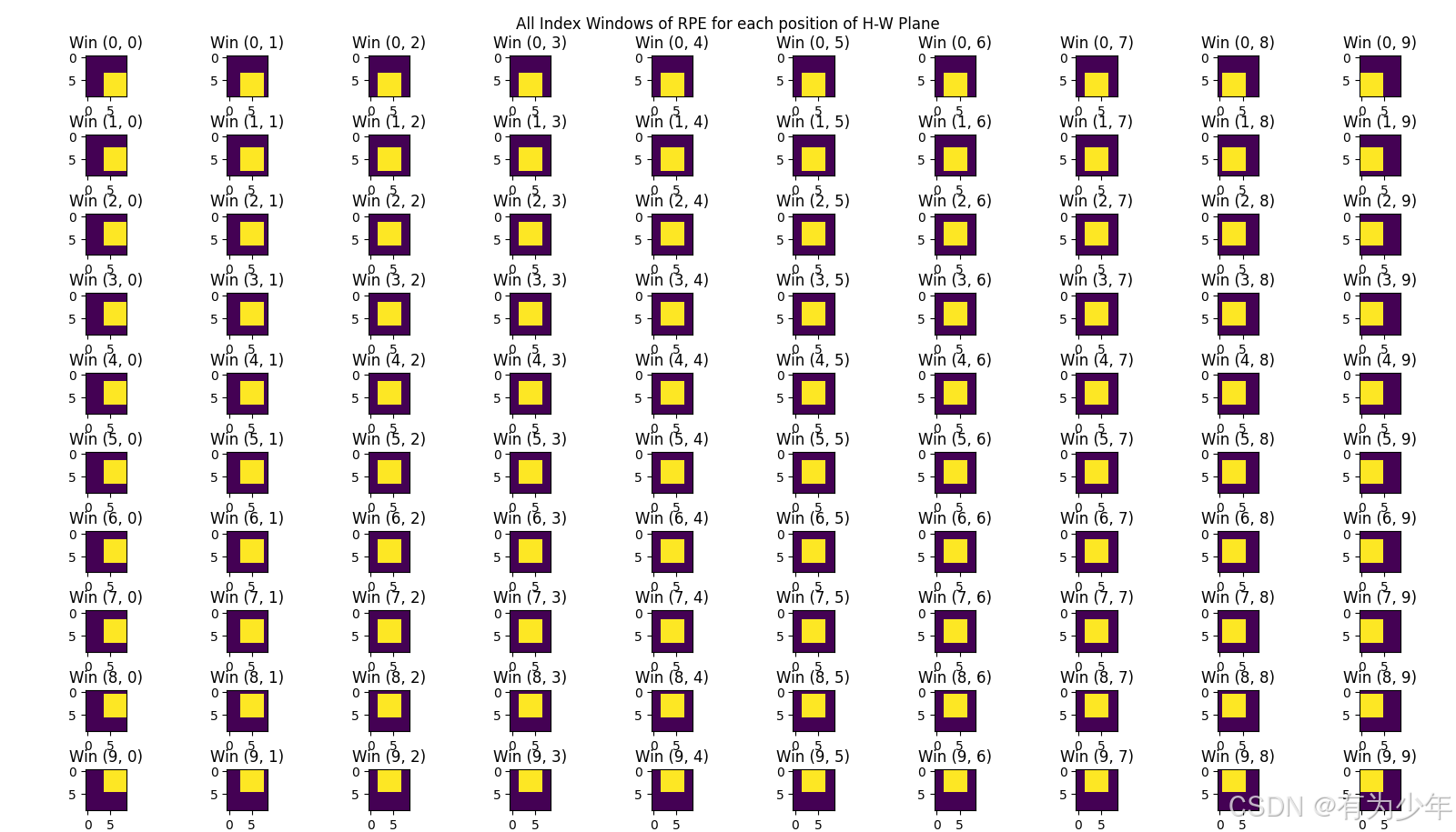
为了便于理解，我在和作者的讨论中重新梳理了这部分内容，并添加了注释：

# specify the height and width of the feature map
height = width = 10

# construct a figure containing height*width subfigures corresponding to different (h,w) pixel
fig, axes = plt.subplots(nrows=height, ncols=width, figsize=(8, 8))
fig.suptitle('All Index Windows of RPE for each position of H-W Plane')

# specify the size of kernel for position bias
kernel_size = 5

# construct a shared relative position bias map
rpb_size = 2 * kernel_size - 1
shared_rpb_bg = np.zeros((rpb_size, rpb_size), dtype=np.uint8)

idx_h = torch.arange(0, kernel_size)
idx_w = torch.arange(0, kernel_size)
# absolute 1D indices in the left-top window of the rpe map (2*kernel_size-1, 2*kernel_size-1)
# other window indices can be obtained by adding a new start index on this `idx_k`
idx_k = ((idx_h.unsqueeze(-1) * rpb_size) + idx_w).reshape(-1)

# construct indices of the window in rpe map for each (h,w) pixel
num_repeat_h = torch.ones(kernel_size, dtype=torch.long)
num_repeat_w = torch.ones(kernel_size, dtype=torch.long)
num_repeat_h[kernel_size // 2] = height - (kernel_size - 1)
num_repeat_w[kernel_size // 2] = width - (kernel_size - 1)
# the base h and w of the four edge regions is different from others
bias_hw = idx_h.repeat_interleave(num_repeat_h).unsqueeze(-1) * rpb_size + idx_w.repeat_interleave(num_repeat_w)
# each (h,w) in the H-W plane corresponds to a window of kernel_size*kernel_size containing indices
bias_idx = (bias_hw.unsqueeze(-1) + idx_k).reshape(-1, kernel_size ** 2) # height*width,kernel_size**2

# change the order
bias_idx = torch.flip(bias_idx.reshape(-1, kernel_size ** 2), [0])

# traverse all positions to visualize and highlight their own index window in the shared rpe map
for h in range(height):
    for w in range(width):
        new_rpb_bg = shared_rpb_bg.flatten().copy()

        new_start_idx = h * height + w
        new_rpb_bg[bias_idx[new_start_idx]] = 255  # index the specific window in rpb map
        new_rpb_bg = new_rpb_bg.reshape(rpb_size, rpb_size)
        axes[h, w].imshow(new_rpb_bg)
        axes[h, w].set_title(f"Win {(h,w)}")

plt.show()

可视化结果：

在这里插入图片描述

在 NAT 的实现中有这样一段代码：

# https://github.com/SHI-Labs/Neighborhood-Attention-Transformer/blob/65396d4e569c4d12b7cb7072f94aed53d18c475b/natten/nattentorch2d.py#L93-L94
pd = self.kernel_size - 1
pdr = pd // 2
...
x = x.unfold(1, self.kernel_size, 1).unfold(2, self.kernel_size, 1).permute(0, 3, 4, 1, 2)
x = pad(x, (pdr, pdr, pdr, pdr, 0, 0), 'replicate')

其中对原始特征 unfold 之后在四周重复补齐 pdr 宽度的 0。这样的操作巧妙地让以边缘区域 ( $\le x < (k-1)//2 + 1$ 和 $\le x < W$ ) 共享相同的局部区域。

Bottleneck Transformer 的实现

Bottleneck Transformer的相对位置编码又是另一种实现方式了，具体可见我这里的分析：https://blog.youkuaiyun.com/P_LarT/article/details/117669123

def pair(x):
    return (x, x) if not isinstance(x, tuple) else x

def expand_dim(t, dim, k):
    t = t.unsqueeze(dim = dim)
    expand_shape = [-1] * len(t.shape)
    expand_shape[dim] = k
    return t.expand(*expand_shape)

def rel_to_abs(x):
    b, h, l, _, device, dtype = *x.shape, x.device, x.dtype
    dd = {'device': device, 'dtype': dtype}
    col_pad = torch.zeros((b, h, l, 1), **dd)
    x = torch.cat((x, col_pad), dim = 3)
    flat_x = rearrange(x, 'b h l c -> b h (l c)')
    flat_pad = torch.zeros((b, h, l - 1), **dd)
    flat_x_padded = torch.cat((flat_x, flat_pad), dim = 2)
    final_x = flat_x_padded.reshape(b, h, l + 1, 2 * l - 1)
    final_x = final_x[:, :, :l, (l-1):]
    return final_x

def relative_logits_1d(q, rel_k):
    b, heads, h, w, dim = q.shape
    logits = einsum('b h x y d, r d -> b h x y r', q, rel_k)
    logits = rearrange(logits, 'b h x y r -> b (h x) y r')
    logits = rel_to_abs(logits)
    logits = logits.reshape(b, heads, h, w, w)
    logits = expand_dim(logits, dim = 3, k = h)
    return logits

class RelPosEmb(nn.Module):
    def __init__(self, fmap_size, dim_head):
        super().__init__()
        height, width = pair(fmap_size)
        scale = dim_head ** -0.5
        self.fmap_size = fmap_size
        self.rel_height = nn.Parameter(torch.randn(height * 2 - 1, dim_head) * scale)
        self.rel_width = nn.Parameter(torch.randn(width * 2 - 1, dim_head) * scale)

    def forward(self, q):
        h, w = self.fmap_size

        q = rearrange(q, 'b h (x y) d -> b h x y d', x = h, y = w)
        rel_logits_w = relative_logits_1d(q, self.rel_width)
        rel_logits_w = rearrange(rel_logits_w, 'b h x i y j-> b h (x y) (i j)')

        q = rearrange(q, 'b h x y d -> b h y x d')
        rel_logits_h = relative_logits_1d(q, self.rel_height)
        rel_logits_h = rearrange(rel_logits_h, 'b h x i y j -> b h (y x) (j i)')
        return rel_logits_w + rel_logits_h