


1 简介
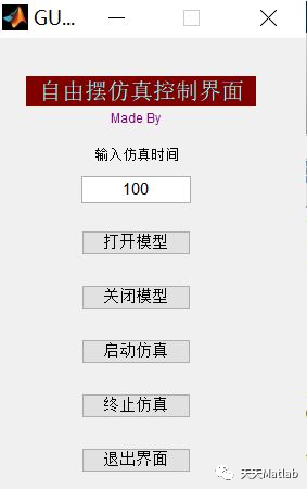
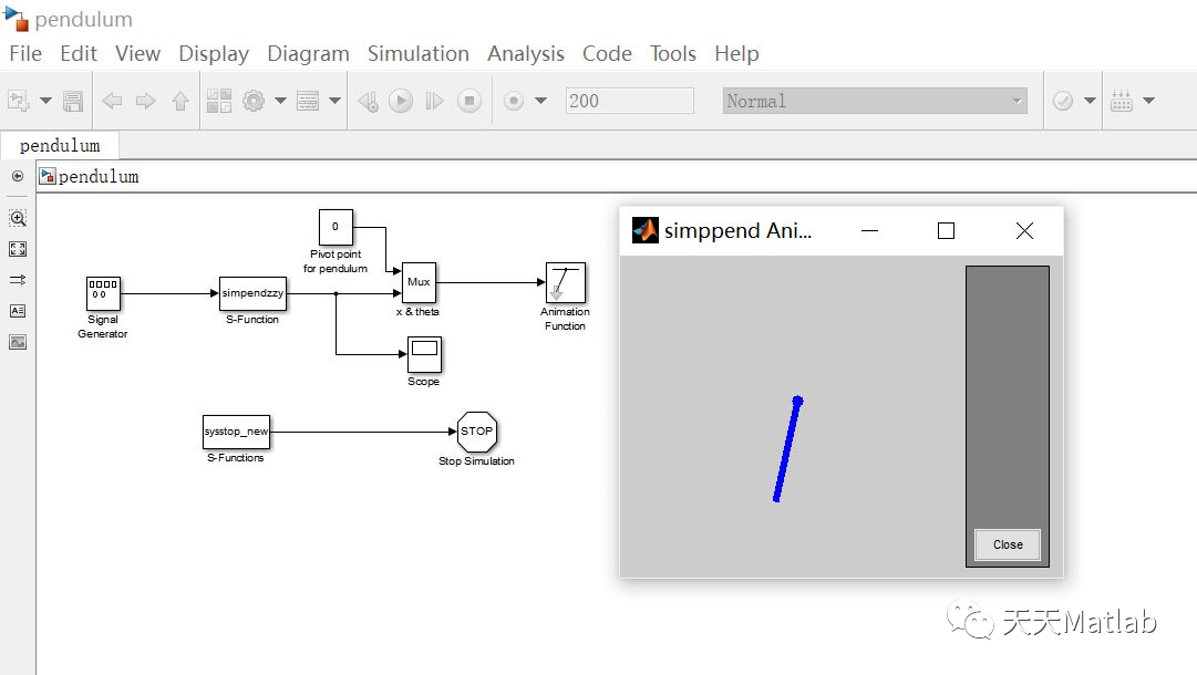
【电路仿真】基于Simulink钟摆自由控制含Matlab源码
2 部分代码
function [sys,x0,str,ts] = simpendzzy(t,x,u,flag,dampzzy,gravzzy,angzzy)
%SFUNTMPL General M-file S-function template
% With M-file S-functions, you can define you own ordinary differential
% equations (ODEs), discrete system equations, and/or just about
% any type of algorithm to be used within a Simulink block diagram.
%
% The general form of an M-File S-function syntax is:
% [SYS,X0,STR,TS] = SFUNC(T,X,U,FLAG,P1,...,Pn)
%
% What is returned by SFUNC at a given point in time, T, depends on the
% value of the FLAG, the current state vector, X, and the current
% input vector, U.
%
% FLAG RESULT DESCRIPTION
% ----- ------ --------------------------------------------
% 0 [SIZES,X0,STR,TS] Initialization, return system sizes in SYS,
% initial state in X0, state ordering strings
% in STR, and sample times in TS.
% 1 DX Return continuous state derivatives in SYS.
% 2 DS Update discrete states SYS = X(n+1)
% 3 Y Return outputs in SYS.
% 4 TNEXT Return next time hit for variable step sample
% time in SYS.
% 5 Reserved for future (root finding).
% 9 [] Termination, perform any cleanup SYS=[].
%
%
% The state vectors, X and X0 consists of continuous states followed
% by discrete states.
%
% Optional parameters, P1,...,Pn can be provided to the S-function and
% used during any FLAG operation.
%
% When SFUNC is called with FLAG = 0, the following information
% should be returned:
%
% SYS(1) = Number of continuous states.
% SYS(2) = Number of discrete states.
% SYS(3) = Number of outputs.
% SYS(4) = Number of inputs.
% Any of the first four elements in SYS can be specified
% as -1 indicating that they are dynamically sized. The
% actual length for all other flags will be equal to the
% length of the input, U.
% SYS(5) = Reserved for root finding. Must be zero.
% SYS(6) = Direct feedthrough flag (1=yes, 0=no). The s-function
% has direct feedthrough if U is used during the FLAG=3
% call. Setting this to 0 is akin to making a promise that
% U will not be used during FLAG=3. If you break the promise
% then unpredictable results will occur.
% SYS(7) = Number of sample times. This is the number of rows in TS.
%
%
% X0 = Initial state conditions or [] if no states.
%
% STR = State ordering strings which is generally specified as [].
%
% TS = An m-by-2 matrix containing the sample time
% (period, offset) information. Where m = number of sample
% times. The ordering of the sample times must be:
%
% TS = [0 0, : Continuous sample time.
% 0 1, : Continuous, but fixed in minor step
% sample time.
% PERIOD OFFSET, : Discrete sample time where
% PERIOD > 0 & OFFSET < PERIOD.
% -2 0]; : Variable step discrete sample time
% where FLAG=4 is used to get time of
% next hit.
%
% There can be more than one sample time providing
% they are ordered such that they are monotonically
% increasing. Only the needed sample times should be
% specified in TS. When specifying than one
% sample time, you must check for sample hits explicitly by
% seeing if
% abs(round((T-OFFSET)/PERIOD) - (T-OFFSET)/PERIOD)
% is within a specified tolerance, generally 1e-8. This
% tolerance is dependent upon your model's sampling times
% and simulation time.
%
% You can also specify that the sample time of the S-function
% is inherited from the driving block. For functions which
% change during minor steps, this is done by
% specifying SYS(7) = 1 and TS = [-1 0]. For functions which
% are held during minor steps, this is done by specifying
% SYS(7) = 1 and TS = [-1 1].
% Copyright 1990-2002 The MathWorks, Inc.
% $Revision: 1.18 $
%
% The following outlines the general structure of an S-function.
%
switch flag,
%%%%%%%%%%%%%%%%%%
% Initialization %
%%%%%%%%%%%%%%%%%%
case 0,
[sys,x0,str,ts]=mdlInitializeSizes(angzzy);
%%%%%%%%%%%%%%%
% Derivatives %
%%%%%%%%%%%%%%%
case 1,
sys=mdlDerivatives(t,x,u,dampzzy,gravzzy);
%%%%%%%%%%
% Update %
%%%%%%%%%%
case 2,
sys=mdlUpdate(t,x,u);
%%%%%%%%%%%
% Outputs %
%%%%%%%%%%%
case 3,
sys=mdlOutputs(t,x,u);
%%%%%%%%%%%%%%%%%%%%%%%
% GetTimeOfNextVarHit %
%%%%%%%%%%%%%%%%%%%%%%%
% case 4,
% sys=mdlGetTimeOfNextVarHit(t,x,u);
%%%%%%%%%%%%%
% Terminate %
%%%%%%%%%%%%%
case 9,
sys=mdlTerminate(t,x,u);
%%%%%%%%%%%%%%%%%%%%
% Unexpected flags %
%%%%%%%%%%%%%%%%%%%%
otherwise
error(['Unhandled flag = ',num2str(flag)]);
end
% end sfuntmpl
%
%=============================================================================
% mdlInitializeSizes
% Return the sizes, initial conditions, and sample times for the S-function.
%=============================================================================
%
function [sys,x0,str,ts]=mdlInitializeSizes(angzzy)
%
% call simsizes for a sizes structure, fill it in and convert it to a
% sizes array.
%
% Note that in this example, the values are hard coded. This is not a
% recommended practice as the characteristics of the block are typically
% defined by the S-function parameters.
%
sizes = simsizes;
sizes.NumContStates = 2;
sizes.NumDiscStates = 0;
sizes.NumOutputs = 1;
sizes.NumInputs = 1;
sizes.DirFeedthrough = 0;
sizes.NumSampleTimes = 1; % at least one sample time is needed
sys = simsizes(sizes);
%
% initialize the initial conditions
%
x0 = angzzy;
%
% str is always an empty matrix
%
str = [];
%
% initialize the array of sample times
%
ts = [0,0];
% end mdlInitializeSizes
%
%=============================================================================
% mdlDerivatives
% Return the derivatives for the continuous states.
%=============================================================================
%
function sys=mdlDerivatives(t,x,u,dampzzy,gravzzy,angzzy)
dx(1)=-dampzzy*x(1)-gravzzy.*sin(x(2))+u;
dx(2)=x(1);
sys = dx;
% end mdlDerivatives
%
%=============================================================================
% mdlUpdate
% Handle discrete state updates, sample time hits, and major time step
% requirements.
%=============================================================================
%
function sys=mdlUpdate(t,x,u)
sys = [];
% end mdlUpdate
%
%=============================================================================
% mdlOutputs
% Return the block outputs.
%=============================================================================
%
function sys=mdlOutputs(t,x,u)
sys = x(2);
% end mdlOutputs
%
%=============================================================================
% mdlGetTimeOfNextVarHit
% Return the time of the next hit for this block. Note that the result is
% absolute time. Note that this function is only used when you specify a
% variable discrete-time sample time [-2 0] in the sample time array in
% mdlInitializeSizes.
%=============================================================================
%
% function sys=mdlGetTimeOfNextVarHit(t,x,u)
%
% sampleTime = 1; % Example, set the next hit to be one second later.
% sys = t + sampleTime;
%
% % end mdlGetTimeOfNextVarHit
%
%=============================================================================
% mdlTerminate
% Perform any end of simulation tasks.
%=============================================================================
%
function sys=mdlTerminate(t,x,u)
sys = [];
% end mdlTerminate
3 仿真结果
4 参考文献
[1]甘雨龙. "自由摆的平板控制系统设计." 物理实验 6(2012):2.
博主简介:擅长智能优化算法、神经网络预测、信号处理、元胞自动机、图像处理、路径规划、无人机等多种领域的Matlab仿真,相关matlab代码问题可私信交流。
🎈 部分理论引用网络文献,若有侵权联系博主删除
🎁 关注我领取海量matlab电子书和数学建模资料
👇 私信完整代码和数据获取及论文数模仿真定制
1 各类智能优化算法改进及应用
生产调度、经济调度、装配线调度、充电优化、车间调度、发车优化、水库调度、三维装箱、物流选址、货位优化、公交排班优化、充电桩布局优化、车间布局优化、集装箱船配载优化、水泵组合优化、解医疗资源分配优化、设施布局优化、可视域基站和无人机选址优化、背包问题、 风电场布局、时隙分配优化、 最佳分布式发电单元分配、多阶段管道维修、 工厂-中心-需求点三级选址问题、 应急生活物质配送中心选址、 基站选址、 道路灯柱布置、 枢纽节点部署、 输电线路台风监测装置、 集装箱船配载优化、 机组优化、 投资优化组合、云服务器组合优化、 天线线性阵列分布优化、CVRP问题、VRPPD问题、多中心VRP问题、多层网络的VRP问题、多中心多车型的VRP问题、 动态VRP问题、双层车辆路径规划(2E-VRP)、充电车辆路径规划(EVRP)、油电混合车辆路径规划、混合流水车间问题、 订单拆分调度问题、 公交车的调度排班优化问题、航班摆渡车辆调度问题、选址路径规划问题
2 机器学习和深度学习方面
2.1 bp时序、回归预测和分类
2.2 ENS声神经网络时序、回归预测和分类
2.3 SVM/CNN-SVM/LSSVM/RVM支持向量机系列时序、回归预测和分类
2.4 CNN/TCN卷积神经网络系列时序、回归预测和分类
2.5 ELM/KELM/RELM/DELM极限学习机系列时序、回归预测和分类
2.6 GRU/Bi-GRU/CNN-GRU/CNN-BiGRU门控神经网络时序、回归预测和分类
2.7 ELMAN递归神经网络时序、回归\预测和分类
2.8 LSTM/BiLSTM/CNN-LSTM/CNN-BiLSTM/长短记忆神经网络系列时序、回归预测和分类
2.9 RBF径向基神经网络时序、回归预测和分类


 897
897

 被折叠的 条评论
为什么被折叠?
被折叠的 条评论
为什么被折叠?
 到【灌水乐园】发言


