tb5_Diving Deep w Table Calculations_data densification平铺_addressing(direction)_partitioning(scope)

Table Calculations are one of the most powerful features in Tableau. They enable solutions that really couldn't be achieved any other way (short of writing a custom application or complex custom SQL scripts!). The features include the following:

• They make it possible to use data that isn't structured well and still get quick results without waiting for someone to fix the data at the source

• They make it possible to compare and perform calculations on aggregate values across rows of the resulting table

• They open incredible possibilities for analysis and creative approaches to solving problems, highlighting insights, or improving the user experience

     Table Calculations range in complexity from incredibly easy to create (a couple of clicks) to extremely complex (requiring an understanding of addressing, partitioning, and data densification[densɪfɪˈkeɪʃn]加密). We'll start off simple and move toward complexity in this chapter. The goal is to gain a solid foundation for creating and using Table Calculations, understanding how they work, and looking at some examples of how they can be used. We'll consider these topics:

• An overview of Table Calculations

• Quick Table Calculations

• Scope and direction

• Addressing and partitioning

• Custom Table Calculations

• Practical examples

• Data densification

     The examples in this chapter will return to the sample Superstore data that we used in the first chapter. To follow along with the examples, use the Chapter 05 Starter.twbx workbook.

An overview of Table Calculations

     Table Calculations are different from all other calculations in Tableau. Row-level, aggregate calculations, and LOD expressions(Level of detail calculations), which we considered in the previous chapterhttps://blog.youkuaiyun.com/Linli522362242/article/details/123188872, are performed as part of the query to the data source. If you were to examine the queries sent to the data source by Tableau, you'd find the code for your calculations translated into whatever flavor of SQL the data source used.

     Table Calculations, on the other hand, are performed after the initial query. Here's an extended diagram that shows how aggregated results are stored in Tableau's cache:
     Table Calculations are performed on the aggregate table of data in Tableau's cache right before the data visualization is rendered. As we'll see, this is important to understand for multiple reasons, including the following:

• Aggregation: Table Calculations operate on aggregate data. You cannot reference fields in a Table Calculation without referencing it as an aggregate.

• Filtering: Regular filters will be applied before Table Calculations. This means that Table Calculations will only be applied to data returned from the source to the cache. You'll need to avoid filtering any data necessary for Table Calculations to work as desired.

• Late Filtering: Table Calculations used as filters will be applied after the aggregate results are returned from the data source. 用作过滤器的表计算将在聚合结果 从数据源返回后 应用The order becomes important: row-level and aggregate filters are applied first, the aggregate data is returned to the cache, then the Table Calculation is applied as a filter that effectively hides data from the view.
  This allows for some creative approaches to solving certain kinds of problems that we'll consider in some of the examples.

• Performance: If you are using a live connection to an enterprise database server, then row-level and aggregate-level calculations will be taking advantage of enterprise-level hardware. Table Calculations are performed in the cache, which means they will be performed on whatever machine is running Tableau. You will not likely need to be concerned if your Table Calculations are operating on a dozen or even hundreds of rows of aggregate data, or if you anticipate publishing to a powerful Tableau Server. However, if you are getting back hundreds of thousands of rows of aggregate data on your local machine, then you'll need to consider the performance of your Table Calculations. At the same time, there are cases where Table Calculations might be used to avoid an expensive filter or calculation at the source.

Creating and editing Table Calculations

There are several ways to create Table Calculations in Tableau, including:

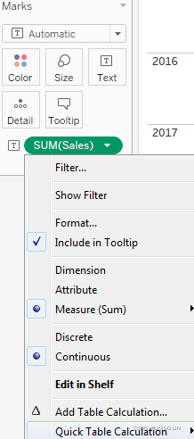
• Using the drop-down menu for any active field used as a numeric aggregate in the view, select Quick Table Calculation and then the desired calculation type

• Using the drop-down menu for any active field that is used as a numeric aggregate in the view, select Add Table Calculation, then select the calculation type, and adjust any desired settings

• Create a calculated field and use one or more Table Calculation functions to write your own custom Table Calculations

     The first two options create a Quick Table Calculation, which can be edited or removed using the drop-down menu on the field and selecting Edit Table Calculation... or Clear Table Calculation. The third option creates a calculated field, which can be edited or deleted as any other calculated field.

     A field on a shelf in the view that is using a Table Calculation, or which is a calculated field using Table Calculation functions, will have a delta symbol icon as follows:

Following is the snippet of Active Field: 

Following is the Active Field with Table Calculation:

     Most of the examples in this chapter will utilize text tables/cross tab reports as these most closely match the actual aggregate table in the cache. This makes it easier to see how the Table Calculations are working.

Tip

     Table Calculations can be used in any type of visualization. However, when building a view that uses Table Calculations, especially more complex ones, try using a table with all dimensions on the Rows shelf and then adding Table Calculations as discrete values on Rows to the right of the dimensions. Once you have all the Table Calculations working as desired, you can rearrange the fields in the view to give you the appropriate visualization.

Quick Table Calculations

     Quick Table Calculations are predefined Table Calculations that can be applied to any field used as a measure in the view. These calculations include common and useful calculations such as running total, difference, percent difference, percent of total, rank, percentile, moving average, YTD total, compound growth rate, Year over Year Growth, and YTD growth. You'll find applicable options on the drop-down list on a field used as a measure in the view, as shown in the following screenshot:
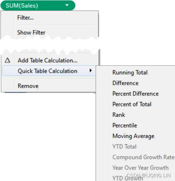
Quick Table Calculations | Runing Total
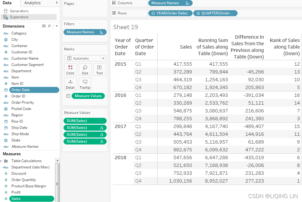
Consider the following example using the sample Superstore Sales data:
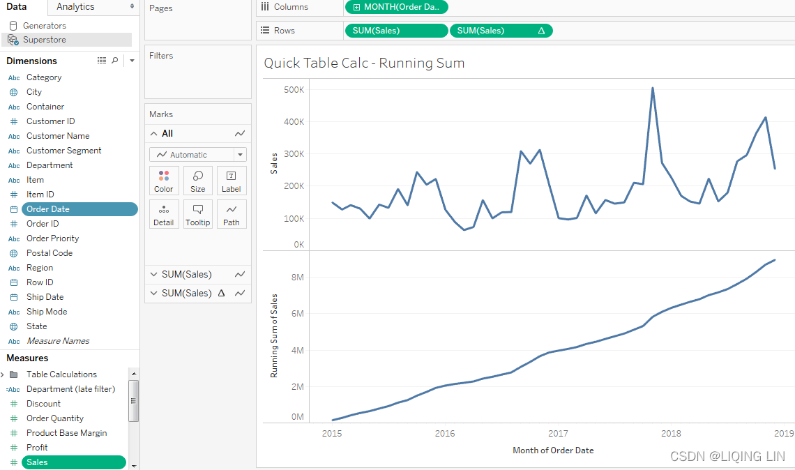
     Here, Sales over time are shown. Sales has been placed on the Rows shelf twice and the second SUM(Sales) field has had the Running Total Quick Table Calculation applied(accumulation of sales). Using the Quick Table Calculation avoided writing any code.

Tip

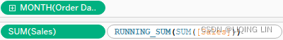
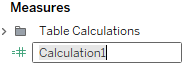
     You can actually see the code that the Quick Table Calculations uses by double-clicking the Table Calculation field in the view. This turns it into an ad hoc calculation. You can also drag an active field with a Quick Table Calculation applied to the data pane, which will turn it into a calculated field available to reuse in other views.

The following table demonstrates some of the Quick Table Calculations available:

• double click Sales under the Measures, then click 
  Running Total==>
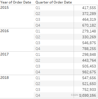
  ==>accumulation of sales==>

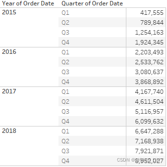
• double click Sales under the Measures, then click Quick Table Calculations | Difference

• double click Sales under the Measures, then click Quick Table Calculations | Rank

• double click Sales under the Measures, then rearrange the fields in the view

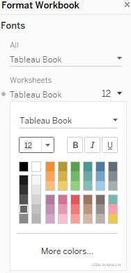
• On the Format menu, select Workbook.
  

Relative versus fixed

     We'll take a look at some of the options for Table Calculations shortly. Based on the options, you can compute Table Calculations in one of the two following ways:

• Relative: The Table Calculation will be computed relative to the layout of the table. They might move across or down the table. Rearranging dimensions in a way that changes the table will change the Table Calculation results. As we'll see, the key for relative Table Calculations is scope and direction. When you set a Table Calculation to use a relative computation, it will continue to use the same relative scope and direction, even if you rearrange the view.

• Fixed: The Table Calculation will be computed using one or more dimensions. Rearranging those dimensions will not change the computation of the Table Calculation. Here the scope and direction remain fixed to one or more dimensions, no matter where they are moved within the view. When we talk about fixed Table Calculations, we'll focus on the concepts of partitioning and addressing.

     You can see these concepts in the user interface. The following is the Table Calculation editor that appears when you select Edit Table Calculation from the menu of a Table Calculation field:

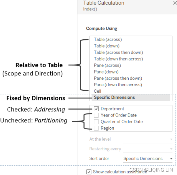
     We'll explore the options and terms in more detail, but for now, notice the options that relate to specifying a Table Calculation that is computed relative to Rows and Columns, and options that specify a Table Calculation that is computed fixed to certain dimensions in the view. 

Scope and direction

     Scope and direction are terms that describe how a Table Calculation is computed relative to the table. When a Table Calculation is relative to the layout of the table, rearranging the fields in the view will not change the scope and direction:

• Scope: The scope defines the boundaries within which a given Table Calculation can reference other values

• Direction: The direction defines how the Table Calculation moves within the scope

     You've already seen Table Calculations being calculated table (across) (the running sum of sales over time销售额随时间的运行总和) and table (down) (in the previous table). In these cases, the scope was the entire table and the direction was either across or down. For example, the running total calculation ran across the entire table, adding subsequent values as it moved from left to right.

     To define scope and direction for a Table Calculation, use the drop-down menu for the field in the view and select Compute Using. You will get a list of options that will vary slightly depending on the location of dimensions in the view. The first of the options listed allows you to define the scope and direction relative to the table. After the option for cell, you will see a list of dimensions present in the view. We'll take a look at those in the next section.

Tip

Options for scope and direction relative to the table:

• Scope options: Table, pane, and cells

• Direction options: Down, across, down then across, across then down

In order to understand these options, consider the following example:
     we've only kept the East and West regions

When it comes to the scope of Table Calculations, Tableau makes the following distinctions:

• The table is the entire set of aggregate data.

• The pane is a smaller section of the entire table. Technically, it is defined by the penultimate[pəˈnʌltɪmət]倒数第二的 lowest level of the table; that is, the next-to-last dimension on the Rows and/or Columns shelf defines the pane. In the preceding image, you can see that the intersection of Year on Rows and Region on Columns defines the panes (one is highlighted, but there are actually 8 panes in the view).

• The cell is defined by the lowest level of the table. In this view, the intersection of one Department within a Region and one Quarter within a Year is a single cell (one is highlighted, but there are actually 96 = 12*8 cells in the view).

     The bounded areas in the preceding screenshot are defined by the scope. Scope (and as we'll see, also partition) defines windows within the data that contain various Table Calculations. Window functions, such as WINDOW_SUM() in particular, work within the scope of a window.

Working with scope and direction

     In order to see how scope and direction work together, let's work through a few examples. We'll start by creating our own custom Table Calculations. Create a new calculated field named Index with the code Index(). 

Tip

     Index() is a Table Calculation function that starts with the value of 1 and increments by one as it moves along a given direction and within a given scope. There are many practical uses for Index, but we'll use it here because it is easy to see how it is moving for a given scope and direction.

     Create the table as shown previously with YEAR(Order Date) and QUARTER(Order Date) on Rows and Region and Department on Columns. Instead of placing Sales in the view, add the newly created Index field to the Text shelf. Then experiment, using the drop-down menu on the Index field and select Compute Using to cycle through various scope and direction combinations. In the following examples, we've only kept the East and West regions and 3 years ( Hide field labels for row by right-click top left cell ):
for example:Pane (across then down)

• Table (across): This is Tableau's default when there are columns in the table. Notice in the following how Index increments across the entire table:
  Compute Using : Cell
  
  ==>Compute Using : Table (across) ; Quick Table Calculation | running total

• Table (down): When using table (down), Index increments down the entire table:

• Table (across then down): This increments Index across the table, then steps down, continues to increment across, and repeats for the entire table:

• Pane (across): This defines a boundary for Index and causes Index to increment across until it reaches the pane boundary, at which point the indexing restarts:

   Compute Using : Cell
  
  ==>Compute Using : Pane (across) ; Quick Table Calculation | running total

• Pane (down): This defines a boundary for Index and causes Index to increment down until it reaches the pane boundary, at which point the indexing restarts:

   Compute Using : Cell ;
  
  ==>Compute Using : Pane (down) ; Quick Table Calculation | running total
  OR
  Compute Using : Cell ;
  
  ==>Compute Using : Pane (down) ; Quick Table Calculation | Percent Difference

   

• Pane (across then down): This allows Index to increment across the pane and continue by stepping down. The pane defines the boundary here:

     You may use scope and direction with any Table Calculation. Consider how a running total or percentage difference would be calculated using the same movement and boundaries shown here. Keep experimenting with different options until you feel comfortable with how scope and direction work. 

     Scope and direction operate relative to the table, so you can rearrange fields, and the calculation will continue to work in the same scope and direction. For example, you could swap Year of Order Date with Department and still see Index calculated according to the scope and direction you defined. 

same with 

 

Addressing and partitioning

     Addressing and partitioning are very similar to scope and direction, but are most often used to describe how Table Calculations are computed with absolute reference to certain fields in the view. With addressing and partitioning, you define which dimensions in the view define the addressing (direction) and all others define the partitioning (scope).

     Using addressing and partitioning gives you much finer control because your Table Calculations are no longer relative to the table layout, and you have many more options for fine-tuning the scope, direction, and order of the calculations.

     To begin to understand how this works, let's consider a simple example. Using the preceding view, select Edit Table Calculation​ from the drop-down menu of the Index(​Compute Using : Table (across) ) field on Text. In the resulting dialog box, check Department under Specific Dimensions.

Here is the result of selecting Department:
​     You'll notice that Tableau is computing Index along (in the direction of) the checked dimension, Department. In other words, you have used Department for addressing, so each new department increments the index. All other unchecked dimensions in the view are implicitly used for partitioning; that is, they define the scope or boundaries at which the index function must restart. As we saw with scope, these boundaries are sometimes referred to as a window.

     The preceding view looks identical to what you would see if you set Index to compute using Pane (across). However, there is a major difference.

• When you use Pane (across), Index is always computed across the pane, even if you rearrange the dimensions in the view, remove some, or add others.

• But when you compute using a dimension for addressing, the Table Calculation will always compute using that dimension. Removing that dimension will break the Table Calculation (the field will turn red with an exclamation mark) and you'll need to edit the Table Calculation via the drop-down menu to adjust the settings. If you rearrange dimensions in the view, Index will continue to be computed along the Department dimension.​

Here, for example, is the result of clicking the Swap Rows and Columns button in the toolbar:
​
     Notice that Index continues to be computed along Department even though the entire orientation of the table has changed. To complete the following examples, we'll undo​ the swap of Rows and Columns to return our table to its original orientation.

Advanced addressing and partitioning

     Let's take a look at a few other examples of what happens when you add additional dimensions. For example, if you check Quarter of Order Date, you'll see Tableau highlight a partition defined by Region and Year of Order Date, with Index incrementing by the addressing fields of Quarter of Order Date and then Department. 

     If you were to select Department and Year of Order Date as the addressing of Index , you'd see a single partition defined by Region and Quarter , like this:
reorder the dimensions by dragging and dropping within the checkbox list of Specific Dimensions:
     You'll notice, in this view, that Index increments for every combination of Year and Department within the partition of Quarter and Region 

     These are a few of the other things to consider when working with addressing and partitioning:

• You can specify the sort order. For example, if you wanted Index to increment according to the value of the sum of sales, you could use the drop-down list at the bottom of the Table Calculation editor to define a custom sort.
• The At the Level option in the edit Table Calculation dialog box allows you to specify a level at which the Table Calculations are performed. Most of the time, you'll leave this set at Deepest (which is the same as setting it to the bottom-most dimension与将其设置为最底部维度相同), but occasionally, you might want to set it at a different level if you need to keep certain dimensions from defining the partition but need the Table Calculation to be applied at a higher level. You can also reorder the dimensions by dragging and dropping within the checkbox list of Specific Dimensions.
• The Restarting Every... option有效地使选定的字段以及选定该字段上方的寻址中的所有维度(here only Year of Order Date)成为分区的一部分 effectively makes the field selected, and all dimensions in the addressing above that field selected, part of the partition, but allows you to maintain the fine-tuning of the ordering.
• Dimensions are the only kinds of fields that can be used in addressing;
  
       however, a discrete (blue) measure can be used to partition Table Calculations. To enable this, use the drop-down menu on the field and uncheck Ignore in Table Calculations. 

Custom Table Calculations

     Before we move on to some practical examples, let's briefly consider how you can write your own Table Calculations, instead of using Quick Table Calculations. You can see a list of available Table Calculation functions by creating a new calculation and selecting Table Calculation from the drop-down list under Functions.

     For each of the examples, we'll setCompute Using | Category. This means Department will be the partition.

     You can think of Table Calculations broken down into several categories. The following Table Calculations can be combined and even nested just like other functions.

Meta table functions

     These are the functions that give you information about the partitioning and addressing. These functions also include Index, First, Last, and Size:All Functions (Categorical) - Tableau

• Index gives an increment as it moves along the addressing within the partition.
• First gives the offset from the first row in the partition; so the first row in each partition is 0.
• Last gives the offset to the last row in the partition; so the last row in each partition is 0.
• Size gives the size of the partition.

The following image shows the various functions:     Index, First, and Last are all affected by scope/partition and direction/addressing, while Size will give the same result at each address of the partition, no matter what direction is specified.

Lookup and previous value

     The first of these two functions gives you the ability to reference values in other rows, while the second gives you the ability to carry forward values. Notice from the following screenshot that direction is very important for these two functions:     Both calculations are computed using an addressing of Category (so Department is the partition).

     Here, we've used the code Lookup(ATTR([Category] ) , -1) , which looks up the value of the category in the row offset by -1 from the current one. The first row in each partition gets a NULL result from the lookup (because there isn't a row before it).

For Previous_Value , we used this code:

Previous_Value("") + ", " + ATTR([Category] )

     Notice that in the first row of each partition, there is no previous value, so Previous_Value() simply returned what we specified as the default: an empty string. This was then concatenated together with a comma and the category in that row, giving us the value, Bookcases.

     In the second row, Bookcases is the previous value, which gets concatenated with a comma and the category in that row, giving us the value, Bookcases, Chairs & Chairmats, which becomes the previous value in the next row. The pattern continues throughout the partition and then restarts in the partition defined by the department Office Supplies.

LOOKUP(expression, [offset])

     Returns the value of the expression in a target row, specified as a relative offset from the current row. Use FIRST() + n and LAST() - n as part of your offset definition for a target relative to the first/last rows in the partition. If offset is omitted, the row to compare to can be set on the field menu. This function returns NULL if the target row cannot be determined.     

     The view below shows quarterly sales. When LOOKUP(SUM(Sales), 2) is computed within the Date partition, each row shows the sales value from 2 quarters into the future.

PREVIOUS_VALUE(expression)

     Returns the value of this calculation in the previous row. Returns the given expression if the current row is the first row of the partition.

Example

SUM([Profit]) * PREVIOUS_VALUE(1) computes the running product of SUM(Profit).

Running functions

     For each of the examples, we'll setCompute Using | Category. This means Department will be the partition. 

     These functions run along the direction/addressing and include Running_Avg() , Running_Count() , Running_Sum() , Running_Min() , and Running_Max() , as follows:     Notice that Running_Sum(SUM[Sales] ) continues to add the sum of sales to a running total for every row in the partition （accumulate）. Running_Min() keeps the value of the sum of sales if it is the smallest value it has encountered so far as it moves along the rows of the partition.

Window functions

WINDOW_SUM(expression, [start, end]) 

     Returns the sum of the expression within the window. The window is defined by means of offsets from the current row. Use FIRST()+n and LAST()-n for offsets from the first or last row in the partition. If the start and end are omitted, the entire partition is used.

     For example, the view below shows quarterly sales. A window sum computed within the Date partition returns the summation of sales across all quarters.

WINDOW_MAX(expression, [start, end])

     Returns the maximum of the expression within the window. The window is defined by means of offsets from the current row. Use FIRST()+n and LAST()-n for offsets from the first or last row in the partition. If the start and end are omitted, the entire partition is used.

     For example, the view below shows quarterly sales. A window maximum within the Date partition returns the maximum sales across all dates. 

     These functions operate across all rows in the partition at once and essentially aggregate the aggregates. They include Window_Sum, Window_Avg, and Window_Max, Window_Min, among others, as shown in the following screenshot:

     For each of the examples, we'll set Compute Using | Category. This means Department will be the partition.

Rank functions

RANK(expression, ['asc' | 'desc'])

     Returns the standard competition rank for the current row in the partition. Identical values are assigned an identical rank. Use the optional 'asc' | 'desc' argument to specify ascending or descending order. The default is descending.

     With this function, the set of values (6, 9, 9, 14) would be ranked (4, 2, 2, 1).

     Nulls are ignored in ranking functions. They are not numbered and they do not count against the total number of records in percentile rank calculations.

     For information on different ranking options, see Rank calculation.

     For each of the examples, we'll set Compute Using | Category. This means Department will be the partition.

Script functions

     These functions allow for integration with the R analytics platform or Python, either of which can incorporate simple or complex scripts for everything from advanced statistics to predictive modeling. It's beyond the scope of this book to dive into all that is possible, but examples are readily available on Tableau's website and from various members of the Tableau community.

All Functions (Categorical) - Tableau

The Total function

    The Total function deserves its own category because it functions a little differently from
the others. Unlike the other functions that work on the aggregate table in the cache, Total
will re-query the underlying source for all the source data rows that make up a given
partition. In most cases, this will yield the same result as a window function.

Practical examples

     Having looked at some of the essential concepts of Table Calculations, let's consider some practical examples. We'll look at several examples, although the practical use of Table Calculations is nearly endless. You are able to do everything from running sums, analyzing year-over-year growth, viewing percentage difference between categories, and much more.

Year over Year Growth

     Often, you may want to compare year over year values. How much has our customer base grown over last year? How did sales in each quarter compare to sales in the same quarter last year? These types of questions can be answered using Year over Year Growth.

      Tableau exposes Year over Year Growth as one option in the Quick Table Calculations. Here, for example, is a view that demonstrates Sales by QUARTER , along with the percentage difference in sales for a quarter compared with the previous year(Quick Table Calculation|Year over Year Growth in

•   and
• ):

     The second Sum(Sales) field has had the Year over Year Growth Quick Table Calculation applied (and the mark type changed to bar). You'll notice the >4 nulls indicator in the lower right, alerting you to the fact that there are at least four null values (which makes sense as there is no 2015 with which to compare quarters in 2016). If you filtered out 2015, the nulls would appear in 2016 as Table Calculations can only operate on values present in the aggregated data in the cache. Any regular filters applied to the data are applied at the source and the excluded data never makes it to the cache.

     As easy as it is to build a view like this example, take care, because Tableau assumes each year in the view has the same number of quarters. For example, if the data for Q1 in 2015 was not present or filtered out, then the resulting view would not necessarily represent what you want. Consider the following, for example:     The problem here is that Tableau is calculating the Quick Table Calculation using an addressing of Year and Quarter and an At the Level of value of Year of Order Date. This works assuming all quarters are present. However, here the first quarter in 2016 is matched with the first quarter present in 2015, which is really Q2. To solve this, you would need to edit the Table Calculation(

•   and
• ):

) to only use Year for addressing. Quarter then becomes the partition and thus comparisons are done for the correct quarter.
==>

     So what if you don't want to show 2015? Filtering it will cause issues for 2016. We'll look at Late Filtering later in this section. Another potential way to remove 2015 is to right-click the 2015 header in the view and select Hide. Hide is a special command that simply keeps Tableau from rendering data, even when it is present in the cache. If you later decide you want to show 2015 after hiding it, you can use the menu for the YEAR(Order Date) field and select Show Hidden Data. Alternately, you can use the menu to select Analysis | Reveal Hidden Data. 

Tip

     You may also wish to hide the null indicator in the view. You can do this by right-clicking the indicator and selecting Hide Indicator. Clicking the indicator will reveal options to filter the data or display it as a default value (typically, 0).

Dynamic titles with totals 

     You've likely noticed the titles that are displayed for every view. There are also captions that are not shown unless you specifically turn them on (to do this, select Worksheet | Show Caption from the menu). 

     By default, the title displays the sheet name and captions are hidden, but you can show and modify each. At times, you might want to display totals that help your end users understand the broad context or immediately grasp the magnitude. 

     Here, for example, is a view that allows the user to select one or more Region and then see Sales per State in each Region
 

     It might be useful to show a changing number of states as the user selects different regions. You might first think to use an aggregation on State , such as Count Distinct. However, if you try showing that in the Title, you will always see the value 1. Why? Because the view level of detail is State and the distinct count of states per state is 1!

     But there are some options with Table Calculations that let you further aggregate aggregates. Or, you might think of determining the number of values in the table based on the size of the window. In fact, here are several possibilities:

• To get the total distinct count: TOTAL(COUNTD([State] ) )
    New Calculation==>==>==>right Caption==>==>Click Insert  <AGG(TOTAL(COUNTD([State])))> ==>
• To get the min within the window: WINDOW_SUM(MIN(1) )
• To get the size of the window: SIZE()

 

     You may recall that a window is defined as the boundaries determined by Scope or Partition. Whichever possibility we choose, we want to define the window as the entire table. Either a relative computation of Table Down or a fixed computation using all of the dimensions would accomplish this. Here is a view that illustrates a dynamic title and all three options in the caption:

Late filtering

     Let's say you've built a view that allows you to see the percent of total sales for each department. You have already used a Quick Table Calculation on the Sales field to give you the percent of the total. You've also used Department as a filter. But this presents a problem.

     Since Table Calculations are performed after the aggregate data is returned to the cache, the filter on department has already been evaluated at the data source and the aggregate rows don't include any departments excluded by the filter. Thus, the percent of the total will always add up to 100%; that is, it is the percentage of the filtered total, as shown in the following screenshot:

     What if you wanted to see the percentage of the total sales for all departments, even if you want to exclude some from the display? One option is to use a Table Calculation as a filter.

     If you create a calculated field called Department (late filter) with the code LOOKUP(ATTR([Department] ) , 0) and place that on the Filters shelf instead of the Department dimension, then the filter is not applied at the source, the aggregate data is visible to other Table Calculations, and the Table Calculation filter merely hides departments from the final view, as shown in the following screenshot:

ATTR

     You might have noticed the ATTR function used. Remember that Table Calculations require aggregate arguments. ATTR (which is short for attribute) is a special aggregation that

• returns the value of a field if there is only a single value of that field present for a given level of detail
• or a * if there is more than one value.

     To understand this, experiment with a view having both Department and Category on Rows. Using the drop-down menu on the active field in the view, change Category to Attribute . It will display as * because there is more than one category for each department. Then, undo and change Department to Attribute . It will display the department name because there is only one department per category. 

Data densification数据致密化

     Data densification is a broad term that indicates that missing values or records are "filled in". Sometimes, specific terms such as domain padding (filling in missing dates or bin values) or domain completion (filling in missing intersections or dimensional values) are used to specify the type of densification, but here, we'll simply use the term data densification.

     Data with missing values (such as data that doesn't have a record for every single date or only contains records for products that have been ordered, as opposed to all products in inventory) is referred to as sparse data.

     Understanding when Tableau uses data densification and how you can turn it on or turn it off is important as you move toward mastering Tableau. There will be times that Tableau will engage data densification when you don't want it and you'll need to recognize this and be aware of the options to turn it off. Other times, you'll want to leverage data densification to solve certain types of problems or perform certain kinds of analysis.

When and where data densification occurs

     Data densification could take place in the source if you chose to fill in missing data with certain joins, unions, or custom queries. But here, we are focused on data densification that takes place in Tableau after aggregate data is returned from the source. Specifically, under certain circumstances that we'll now consider, Tableau fills in missing values in the aggregate data in the cache, as seen in this diagram:
vs

     You'll recognize this diagram as very similar to the diagram we examined when we started the discussion on Table Calculations. In fact, data densification happens at more or less the same time as Table Calculations, and can sometimes even be triggered by Table Calculations. Here are some examples of times when data densification is enabled: 

• When the Show Missing Values option is enabled for dates or bins used as headers on Rows or Columns. Here, Tableau will show headers for dates or bin values (between the minimum or maximum dates/bin values), even if they don't occur in the data (or are eliminated by a filter). You can easily turn this densification on or off by selecting the desired option.
• With Show Missing Values enabled, certain Table Calculations used in the view will additionally add marks in the view for the missing headers. We'll see an example of this later in this section.
• Using certain Table Calculations with discrete dimensions on Rows and Columns will cause Tableau to turn on data densification.
• Enabling the Show Empty Rows/Columns option (to do this, from the menu, select Analysis | Table Layout | Show Empty Rows/Columns.) This causes Tableau to show all row/column headers, even if particular values wouldn't normally be shown based on filter selections. This option is context-specific, so the domain of values shown is either for the entire dataset, or for the context defined by context filters. Observe the difference between the Categories shown with and without the option checked:

 ==>==>==>==>==>Without Show Empty Rows, only Categories with records for the filtered Region and Month are Visible

 ==>With Show Empty Rows, all Categoreis are shown even if there are no records for the filtered Region and Month

==>Show Empty Rows

Using certain Table Calculations with discrete dimensions on Rows and Columns will cause Tableau to turn on data densification.

     Let's take a look at an example and how to optionally turn off the resulting densification. Observe the difference between the two views, as follows: This view has 14 marks (you can see the count in the status bar), indicating that there are 14 valid intersections of Container and Ship Modes . Some combinations simply don't occur in the data (for example, a Jumbo Drum is never sent by Express Air).

     But adding a Table Calculation such as Index() to the Detail causes Tableau to fill in the missing intersections, like this:
Tableau has filled in the combinations of Container and Ship Mode and there are now 21 marks. Sometimes, this behavior might be useful (and we'll see such an example next), but many times, you may want to avoid the densification. How can you turn it off?

     With an understanding that Tableau has enabled the densification because of the discrete dimensions on Rows and Columns, you can rearrange the view so that only one dimension remains on Rows or Columns. This view, for example, keeps Ship Mode on Detail as part of the view level of detail, but uses the special aggregation ATTR on Columns, as shown in the following screenshot:
The result is a view without data densification showing only 14 marks.

Tip

     Keep an eye on the status bar and the count of marks. This will help you identify possible cases of data densification. You will then be able to decide when you wish to leverage densification or when it is useful to turn it off. 

An example of leveraging data densification 

     Beyond simple examples of showing empty rows or missing dates, there are cases where you can use data densification to solve problems or get around limitations of the data绕过数据的限制 that would be very difficult otherwise否则这些限制将非常困难. 

     Consider, for example, if you had data that indicated dates when certain generators were turned on or off, such as the following, for example:What if you wanted a visualization that showed how many generators were On for any given date? The challenge is that the dataset is sparse. That is, there are only records for dates when an On or Off action occurred. The following shows how easy it is to visualize this in Tableau:

• Exact Date
• Discrete
• 

 We only have 8 marks to work with. But we've already seen that Tableau can fill in missing dates, and additionally, we can further force data densification by using certain Table Calculations to fill in a value for each generator for every date.

     We'll start with a calculation that takes the human friendly value of On or Off and change it to a value we can easily add. The calculation is named Action value, and is used value with the following code:

IF [Action] = "On" THEN 1 ELSE 0 END

 This will give us a 1 to count the generator when it is On , and a 0 otherwise.

     An additional calculation, combined with enabling the Show Missing Values of the Date field, allows us to fill in every date with a value. The new calculated field is called Action Value for Date and has the following code:

IF NOT ISNULL(MIN([Action Value])) 
THEN MIN([Action Value])
ELSE ZN(PREVIOUS_VALUE(MIN([Action Value])))
END

     This implements a Table Calculation that we will set to calculate across the table(Table across).

• If MIN([Action Value] ) is not null, then we have arrived at a date where the data gives an actual value and we'll keep that.
• Otherwise, we'll carry forward the PREVIOUS_VALUE() (a 1 if the generator was turned on or a 0 if it was turned off).
• The ZN() function will turn any null values into 0 (we'll assume the generator is off until we encounter an On ).
• We'll move across the table, carrying forward values until we come across a value present in the data. Then we'll carry that one forward. The result is a table with all dates filled in with values, like this:

 Notice that every generator gets a 1 on the date it was turned on and that 1 is carried across the table until the generator is turned off, at which point we get the 0 and carry it across.

     We're close, because all we have to do now is sum up the values for all generators for a given date to get the number of generators that were on. For example, on day 13, there was only one. On day 25, there were four.

     We can accomplish this using one more calculation that nests our existing calculation. We'll name this calculated field Generators Operating and use the following code:

WINDOW_SUM([Action Value for Date])

     The key here is that we want to sum all the values down the table, but we want those values to be calculated across the table. When you use nested Table Calculations (Table Calculations referenced within the code of other Table Calculations), you can specify the scope/direction or addressing/partitioning for each nested calculation.

     Here, for example, we'll add the Generators Operating calculated field to Rows and use the drop-down menu to select the Edit Table Calculation option:
and

     Observe that under the Nested Calculations heading, there is a drop-down list where you can change the Compute Using options for each nested calculation. Here, we'll set Generators Operating to Table (down) and Action Value for Date to Table (across).

We've cleaned up the view a bit by doing the following:

• We've added a First() == 0 filter, which is computed Table (down) because we're getting the total sum of action values for Date for each generator and we only need to show one set of totals.
  Right-click an empty area on Marks ==> New Calculation ==>==>drag and move it to Filter==>==>Table (down)==>
• We've hidden the column headers for Generator , because the field needs to be in the view to define the view level of detail, but does not need to be shown.
• We've changed the Marks to Area.

Our final view, after a bit of a cleanup, will look something like this: The final view gives us a clear indication of how many generators were on for any given date, even though many of those dates did not exist in the data and we certainly didn't have a record for every generator for every date.

     Would it have been easier or better to densify the data at the source by joining every generator with every date to get a record for each combination? Quite likely. If it is possible, given your data source, to perform such a join, you may end up with a dataset that is far easier to work with in Tableau (without having to use data densification or complex Table Calculations). 

     You'll have to evaluate the feasibility of filling in missing data at the source based on volumes of data, underlying capabilities of the database, and how quickly such transformations can be accomplished. Having an understanding of data densification gives you some options to consider if you don't have the ability to shape the source.

     However, with Tableau Prep, the possibilities for reshaping data easily are often within reach. We'll consider some of these possibilities when we examine Tableau Prep in Chapter 10 , Introducing Tableau Prep.

Summary

      We've covered a lot of concepts surrounding Table Calculations in this chapter. You now have a solid foundation for understanding everything, from Quick Table Calculations to advanced Table Calculations and data densification. The practical examples we covered barely scratch the surface of what is possible, but should give you an idea of what can be achieved. The kinds of problems that can be solved and the diversity of questions that can be answered are almost limitless! 

     We'll turn our attention to some lighter topics in the next couple of chapters, looking at formatting and design, but we'll certainly see another Table Calculation or two before we're finished!