


 本文探讨了深度计算机视觉中的关键概念和技术,包括对象检测、全卷积网络、YOLO算法及其改进版本,以及语义分割等主题。
14_Deep Computer Vision Using Convolutional Neural Networks_pool_GridSpec:
https://blog.youkuaiyun.com/Linli522362242/article/details/108302266
14_Deep Computer Vision Using Convolutional Neural Networks_2_LeNet-5_ResNet-50_ran out of data
https://blog.youkuaiyun.com/Linli522362242/article/details/108396485
https://cs231n.github.io/convolutional-networks/
Object Detection
The task of classifying and localizing multiple objects in an image is called object detection. Until a few years ago, a common approach was to take a CNN(Convolutional Neural Networks) that was trained to classify and locate a single object, then slide it across the image, as shown in Figure 14-24. In this example, the image was chopped into a 6 × 8 grid, and we show a CNN (the thick black rectangle) sliding across all 3 × 3 regions. When the CNN was looking at the top left of the image, it detected part of the leftmost rose, and then it detected that same rose again when it was first shifted one step to the right. At the next step, it started detecting part of the topmost rose, and then it detected it again once it was shifted one more step to the right. You would then continue to slide the CNN through the whole image, looking at all 3 × 3 regions. Moreover, since objects can have varying sizes, you would also slide the CNN across regions of different sizes. For example, once you are done with the 3 × 3 regions, you might want to slide the CNN across all 4 × 4 regions as well.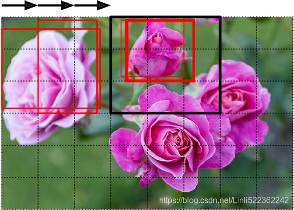 Figure 14-24. Detecting multiple objects by sliding a CNN across the image
This technique is fairly straightforward, but as you can see it will detect the same object multiple times, at slightly different positions. Some post-processing will then be needed to get rid of all the unnecessary bounding boxes. A common approach for this is called non-max suppression. Here’s how you do it:
1. First, you need to add an extra objectness output to your CNN, to estimate the probability that a flower is indeed present in the image (alternatively, you could add a “no-flower” class, but this usually does not work as well). It must use the sigmoid activation function, and you can train it using binary cross-entropy loss. Then get rid of all the bounding boxes for which the objectness score(The objectness score is defined to measure how well the detector identifies the locations and classes of objects during navigation) is below some threshold: this will drop all the bounding boxes that don’t actually contain a flower.
2. Find the bounding box with the highest objectness score, and get rid of all the other bounding boxes that overlap a lot with it (e.g., with an IoU greater than 60%). For example, in Figure 14-24, the bounding box with the max objectness score is the thick bounding box over the topmost rose (the objectness score is represented by the thickness of the bounding boxes). The other bounding box over that same rose overlaps a lot with the max bounding box, so we will get rid of it.
3. Repeat step two until there are no more bounding boxes to get rid of.
This simple approach to object detection works pretty well, but it ![]() requires running the CNN many times
requires running the CNN many times![]() , so it is quite slow. Fortunately, there is a much faster way to slide a CNN across an image: using a fully convolutional network (FCN).
, so it is quite slow. Fortunately, there is a much faster way to slide a CNN across an image: using a fully convolutional network (FCN).
Fully Convolutional Networks
The idea of FCNs was first introduced in a 2015 paper(Jonathan Long et al., “Fully Convolutional Networks for Semantic Segmentation,” Proceedings of the IEEE Conference on Computer Vision and Pattern Recognition (2015): 3431–3440.) by Jonathan Long et al., for semantic segmentation (the task of classifying every pixel in an image according to the class of the object it belongs to). The authors pointed out that you could replace the dense layers at the top of a CNN by convolutional layers.
Local Connectivity
Example 1. For example, suppose that the input volume has size [32x32x3], (e.g. an RGB CIFAR-10 image). If the receptive field (or the filter size) is 5x5, then each neuron in the Conv Layer will have weights to a [5x5x3] region in the input volume, for a total of 5*5*3 = 75 weights (and +1 bias parameter). Notice that the extent of the connectivity along the depth axis must be 3, since this is the depth of the input volume.https://cs231n.github.io/convolutional-networks/#conv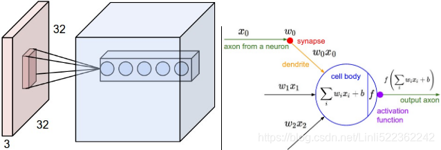 Left: An example input volume in red (e.g. a 32x32x3 CIFAR-10 image), and an example volume of neurons in the first Convolutional layer. Each neuron in the convolutional layer is connected only to a local region in the input volume spatially, but to the full depth (i.e. all color channels). Note, there are multiple neurons (5 in this example) along the depth, all looking at the same region in the input - see discussion of depth columns in text below. Right: The neurons from the Neural Network chapter remain unchanged: They still compute a dot product of their weights with the input followed by a non-linearity(e.g. ReLU), but their connectivity is now restricted to be local spatially.
Example 2. Suppose an input volume had size [16x16x20]. Then using an example receptive field size of 3x3, every neuron in the Conv Layer would now have a total of 3*3*20 = 180 connections to the input volume. Notice that, again, the connectivity is local in space (e.g. 3x3), but full along the input depth (20).
#############
the dense layer’s output was a tensor of shape [batch size, 200]
tensorflow v1
# Implementing a CNN in TensorFlow low-level API by using tensorflow.compat.v1
import tensorflow.compat.v1 as tf
import numpy as np
def fc_layer(input_tensor, # Tensor("Placeholder:0", shape=(None, 7, 7, 100), dtype=float32)
name, # name='fctest'
n_output_units, # n_output_units=200
activation_fn=None):# activation_fn=tf.nn.relu
with tf.variable_scope(name):
input_shape = input_tensor.get_shape().as_list()[1:] # return [7, 7, 100]
n_input_units = np.prod(input_shape) # return 4900 = 7*7*100
# similar to model.add( keras.layers.Flatten() ) # since a dense network expects a 1D array of features for each instance
if len(input_shape) > 1:
input_tensor = tf.reshape(input_tensor,
shape=(-1, n_input_units)
)#Tensor("fctest/Reshape:0", shape=(None,4900), dtype=float32)
weights_shape = [n_input_units, n_output_units] #[4900, 200]
# tf.compat.v1.get_variable
# # Gets an existing variable with these parameters or create a new one.
weights = tf.get_variable(name='_weights',
shape=weights_shape)
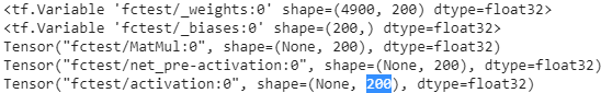
print(weights) # <tf.Variable 'fctest/_weights:0' shape=(4900, 200) dtype=float32>
biases = tf.get_variable(name='_biases',
initializer=tf.zeros(
shape=[n_output_units]
)
)
print(biases) # <tf.Variable 'fctest/_biases:0' shape=(200,) dtype=float32>
# mat_shape(batches, 4900) x mat_shape(4900, 200) ==> mat_shape(batches, 200)
layer = tf.matmul(input_tensor, weights)#shape(None, 200)
print(layer) # Tensor("fctest/MatMul:0", shape=(None, 200), dtype=float32)
layer = tf.nn.bias_add(layer, biases,
name='net_pre-activation')
print(layer) # Tensor("fctest/net_pre-activation:0", shape=(None, 200), dtype=float32)
if activation_fn is None:
return layer
layer = activation_fn(layer, name='activation')
print(layer) # Tensor("fctest/activation:0", shape=(None, 200), dtype=float32)
return layer
## testing:
g = tf.Graph()
with g.as_default():
x = tf.placeholder(tf.float32, shape=[None, 7, 7, 100]) #100 feature maps, each of size 7 × 7 (this is the feature map size
fc_layer(x, name='fctest', n_output_units=200,
activation_fn=tf.nn.relu)
del g, xfor each instance
tensorflow v2
import tensorflow as tf # tf.__version__ : '2.1.0'
from tensorflow import keras
import numpy as np

def fc_layer(input_tensor,       # Tensor("Placeholder:0", shape=(None, 7, 7, 100), dtype=float32)
             name,               # name='fctest'
             n_output_units,     # n_output_units=200
             activation_fn=None):# activation_fn=tf.nn.relu

    # print(input_tensor.get_shape().as_list()) # [None, 7, 7, 100]
    input_shape = input_tensor.get_shape().as_list()[1:] # # print(input_shape) # [7, 7, 100]
    n_input_units = np.prod(input_shape) # return 4900 = 7*7*100

    # similar to model.add( keras.layers.Flatten() ) # since a dense network expects a 1D array of features for each instance
    if len(input_shape) > 1:
        input_tensor = tf.reshape(input_tensor,
                                  shape=(-1, n_input_units)
                                 )
        # print(input_tensor) # Tensor("lambda_7/Reshape:0", shape=(None, 4900), dtype=float32)

    initializer = tf.keras.initializers.RandomNormal(mean=0., stddev=1.)#########
    # tf.Variable :
    #   # The Variable() constructor requires an initial value for the variable,
    #   # which can be a Tensor of any type and shape. This initial value defines the
    #   # type and shape of the variable. After construction, the type and shape of the
    #   # variable are fixed. The value can be changed using one of the assign methods
    weights = tf.Variable( initializer( shape=(n_input_units, n_output_units ) ),
                           name='_weights')#########
    print(weights) # <tf.Variable '_weights:0' shape=(4900, 200) dtype=float32, numpy=


    biases = tf.Variable( initial_value=tf.zeros( shape=n_output_units ),
                          name='_bias')#########
    print(biases) # <tf.Variable '_bias:0' shape=(200,) dtype=float32, numpy=


    layer = tf.matmul(input_tensor, weights)
    print(layer) # Tensor("lambda_6/MatMul:0", shape=(None,  200), dtype=float32)

    # layer=layer+biases # applying broadcasting
    # OR
    layer = tf.nn.bias_add( layer, biases,
                            name='net_pre-activation')
    print(layer) # Tensor("net_pre-activation_11:0", shape=(None, 200), dtype=float32)


    if activation_fn is None:
        return layer

    layer = activation_fn(layer, name='activation') # similar to # tf.keras.activations.get( 'activation' )
    print(layer) # Tensor("lambda_6/activation:0", shape=(None, 200), dtype=float32)
    return layer

x_in = keras.layers.Input(shape=(7,7,100), batch_size=None, name='input')
fc_layer(x_in, name='fctest', n_output_units=200, activation_fn=tf.nn.relu)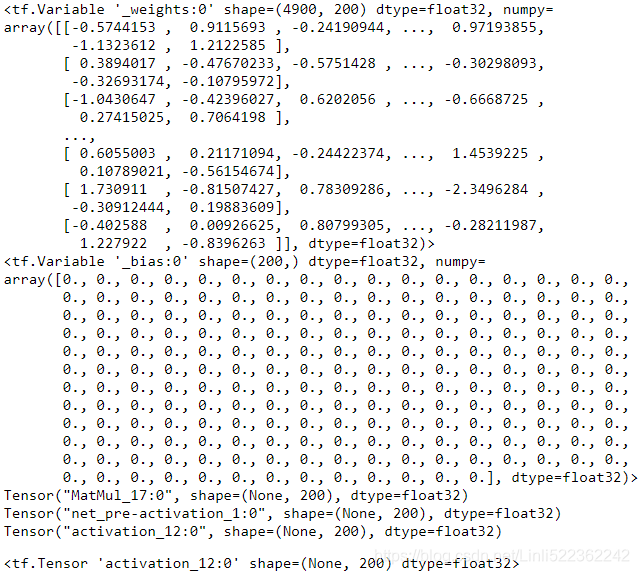
To understand this, let’s look at an example: suppose a dense layer with 200 neurons(n_neurons=200 or C_out=200) sits on top of a convolutional layer that outputs 100 feature maps or channels(is the C_in of this dense layer), each of size 7 × 7 (this is the feature map size(input_tensor), not the kernel size). Each neuron will compute a weighted sum of all 100 × 7×7 activations from the convolutional layer (plus a bias term, 1 bias per neurons or per output chanel or per feature map in C_out ).
###
for this dense layer, 100 channels * input_X.shape(7,7) https://blog.youkuaiyun.com/Linli522362242/article/details/108414534
tf.matmul( input_tensor.shape(batches, 4900), weights.shape=(4900, 200) )==>shape=( batches OR None, 200) +b.shape(200, since 1 bias per neurons or output chanels C_out ) ==>(None, 200)==> 200 numbers
### VS a Convolution layer
#########################################################
Numpy examples. To make the discussion above more concrete, lets express the same ideas but in code and with a specific example. Suppose that the input volume is a numpy array X. Then:
- A depth column (or a fibre) at position
(axis_0,axis_1)would be the activationsX[axis_0,axis_1,:]. - A depth slice, or equivalently an activation map at depth
dwould be the activationsX[:,:,d].
Conv Layer Example. Suppose that the input volume X has shape X.shape: (11,11,4). Suppose further that we use no zero padding (P=0), that the filter size is F=5x5, and that the stride is S=2. The output volume would therefore have spatial size (11+2*0-5)/2+1 = 4, giving a volume with width and height of 4. The activation map in the output volume (call it V), would then look as follows (only some of the elements are computed in this example): W.shape(5,5,C_in=4, C_out)
V[0,0,0] = np.sum(X[:5,:5,:] * W0) + b0(example of going alongaxis_0) and the '*' does element-wise multiplicationV[1,0,0] = np.sum(X[2:7,:5,:] *W0) + b0V[2,0,0] = np.sum(X[4:9,:5,:] *W0) + b0V[3,0,0] = np.sum(X[6:11,:5,:]*W0) + b0
1 bias per neuron or per output chanel in C_outnote np.sum(X[:5,:5,_:_] * W0) ==> sum(X[:5,:5,0]*W0)+sum(X[:5,:5,1]*W0)+sum(X[:5,:5,2]*W0)+sum(X[:5,:5,4-1]*W0) #along deep #C_in=4
Remember that in numpy, the operation * above denotes elementwise multiplication between the arrays. Notice also that the weight vector W0 is the weight vector of that neuron and b0 is the bias. Here, W0 is assumed to be of shape W0.shape: (5,5,4), since the filter size is 5 and the depth of the input volume is 4. Notice that at each point, we are computing the dot product as seen before in ordinary neural networks. Also, we see that we are using the same weight and bias (due to parameter sharing), and where the dimensions along the width are increasing in steps of 2 (i.e. the stride).
To construct a second activation map in the output volume, we would have:
V[0,0,1] = np.sum(X[:5,:5,:] * W1) + b1(example of going alongaxis_0) and the '*' does element-wise multiplicationV[1,0,1] = np.sum(X[2:7,:5,:] * W1) + b1V[2,0,1] = np.sum(X[4:9,:5,:] * W1) + b1V[3,0,1] = np.sum(X[6:11,:5,:]* W1) + b1V[0,1,1] = np.sum(X[:5,2:7,:] * W1) + b1( example of going alongaxis_1 in thesecond activation map)V[2,3,1] = np.sum(X[4:9,6:11,:] * W1) + b1( or along both(axis_0, axis_1) )
where we see that we are indexing into the second depth dimension in V (at index 1) because we are computing the second activation map, and that a different set of parameters (W1) is now used. In the example above, we are for brevity leaving out some of the other operations the Conv Layer would perform to fill the other parts of the output array V. Additionally, recall that these activation maps are often followed elementwise through an activation function such as ReLU, but this is not shown here.
#########################################################
convert the CNN (the last layer is a dense layer) into an convolutional layer or FCN(Fully Convolutional Networks)
To understand this, let’s look at an example: suppose a dense layer with 200 neurons(n_neurons=200 or C_out=200) sits on top of a convolutional layer that outputs 100 feature maps or channels
(###
input_tensor, : Tensor("Placeholder:0", shape=(None, 7, 7, 100), dtype=float32)
###)
,each of size 7 × 7 (this is the feature map size(input_tensor), not the kernel size). Each neuron will compute a weighted sum
(###
layer=tf.matmul(input_tensor.shape=(None, 4900), weights.shape=(4900, 200))
###)
of all 100 × 7×7 activations from the convolutional layer (plus a bias term, 1 bias per neurons or per output chanel or per feature map in C_out )
(###
layer = tf.nn.bias_add( layer, biases.shape=(200,), name='net_pre-activation' )
output.shape : (None_batch size, 200)
###)
. Now let’s see what happens if we replace the dense layer with a convolutional layer using 200 filters(since
 最低0.47元/天 解锁文章


 551
551

 被折叠的 条评论
为什么被折叠?
被折叠的 条评论
为什么被折叠?
 到【灌水乐园】发言


