【船舶定位】粒子滤波算法求解船舶位置问题【含Matlab源码 3496期】

💥💥💥💥💥💥💥💥💞💞💞💞💞💞💞💞💞Matlab武动乾坤博客之家💞💞💞💞💞💞💞💞💞💥💥💥💥💥💥💥💥
🚀🚀🚀🚀🚀🚀🚀🚀🚀🚀🚤🚤🚤🚤🚤🚤🚤🚤🚤🚤🚤🚤🚤🚤🚤🚤🚤🚤🚤🚤🚀🚀🚀🚀🚀🚀🚀🚀🚀🚀

🔊博主简介：985研究生，Matlab领域科研开发者；

🚅座右铭：行百里者，半于九十。

🏆代码获取方式：
优快云 Matlab武动乾坤—代码获取方式

更多Matlab物理应用仿真内容点击👇
①Matlab物理应用（进阶版）

⛳️关注优快云 Matlab武动乾坤，更多资源等你来！！

⛄一、粒子滤波算法求解船舶位置问题

粒子滤波定位算法是目前最精准定位可移动物体的位置，由于水域的流动，工业固体废物污染源很可能随着水流移动位置，基于粒子滤波算法将污染物定位分为预测、测量以及重新采样可大大提高定位准确率[10]。粒子滤波算法的定位过程首先根据水流速度以及前一时刻水域的污染浓度预测出目前水域污染浓度最高的区域，其次对每个可能为污染源的位置进行权重计算，最后将所有污染源权重进行筛选，剔除权值较小的污染源，留下权值最高的污染源，并重复训练直到获取唯一一个权值最高的污染源，即实现工业固体废物污染定位。

1 预测阶段
在此阶段中首先设置出所需粒子个数，并将所有粒子平分到受到污染的水域中，基于粒子滤波算法得出提议分布，当污染源在时间t-1中的定位是Xt-1(xt-1,yt-1,θt-1),则时间t的污染源定位是Xt(xt,yt,θt),污染源的运动速度即为水流速度，则工业固体废物污染源在时间t到t-1之间位置的变化表达式(5)为：

首先利用摄像机和激光扫描仪在水域污染浓度较高的区域进行扫描，假设摄像机以及激光扫描仪获取到的固体点特征角度表达式(6)为：

为将激光扫描仪角度数据与摄像机中的物体角度信息进行中和，需要对摄像机中的物体点角度数据进行旋转变换根据角度信息公式将两种设备之间的角度信息进行转换，且转换时必须满足误差正态分布，则转换表达式(7)为：

根据式(9)将两种设备的废物样本集成到提议分布内，进而使得提议分布函数更加集中，即样本范围更小，更容易对污染源进行定位，此时的提议分布函数表达式(9)为：

上式即为根据状态转移函数得出的粒子滤波状态提议分布。

2 测量阶段
在此阶段直接将激光扫描数据当成输入，进而获取工业固体废物的位置信息，则通过激光扫描仪位置转换生成设备与工业固体废物之间的几何关系表达式(10)为：

式中，xt代表设备的具体位置，θ代表设备扫描物体的角度，d代表设备与观测到的物体之间的直线距离，β代表物体的角度。

在激光数据中获取疑似为工业固体废物污染源的观测值，并对其中的各个粒子进行权重评价，其表达式(11)为：

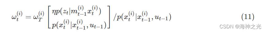
根据粒子的权重判断粒子是否为真的工业固体废物。

3 重采样阶段
根据每个粒子的权重大小决定是否保留该粒子，设置一个可接受范围，判断粒子是否在此范围内，为保证粒子不变，复制权重较大的粒子填补空缺位置，重组粒子后将所有粒子输入状态转移函数内，并反复进行训练，保证最终污染源定位的准确性，实现工业固体废物污染源的定位。

⛄二、部分源代码

%demonstration of particle filtering
%by Paul Sundvall, KTH Signals sensors and systems 2004
clear,clc,close all

%let x be the position of the boat
%create a model for the movement of the boat
xmin=-10;
xmax=10;
xpmin=-.3;
xpmax=.3;
N=10000;
m=1;%kg
kk=1;%N/m
c=.5;%N/s
F0=25;%N
dT=.05;%s
M=400;%timesteps

%first calculate the true sequence of disturbance force
wk=(rand(M,1)-.5)2F0;

af=[1 -2 1].(dT^-2)+[0 kk/m 0]+[1 0 -1]./2/dTc/m;
bf=1/m;
xtrue=filter(bf,af,wk);
xptrue=filter([1 -1]/dT,1,xtrue);

% plot(xtrue)
% title(‘true x’)
% xlabel(‘time step’)
% ylabel(‘x (m)’)
% pause

%calculate the measurement
sigma=.3;%measurent noise std deviation.
a=.2;%constant for the average slope of the bottom surface
b=0;
z=sin(xtrue)+axtrue+bxtrue.*xtrue + randn(M,1)*sigma; %first part is the bottom surface, last term is the measurement noise

%initialization
xk=rand(N,1)*(xmax-xmin)+xmin;
xpk=zeros(N,1);

pik=repmat(1/N,N,1); %the propability that we are in state xk, xpk.
figure(1)
set(1,‘doublebuffer’,‘on’,‘position’,[239 291 681 343])
t=linspace(xmin,xmax,N)';
h1=line(t,sin(t)+at+bt.*t,‘marker’,‘none’);%t is just a temporary variable to draw the bottom surface
h3=line(xtrue(1),0,‘marker’,‘o’,‘linestyle’,‘none’);

%plot the boat
boat.x=[-2.4 -2 -1 0 1 2 2 -2.4]‘;
boat.y=[ 1 0 -.2 -.3 -.3 -.3 .8 1]’+5;
hboat=line(boat.x+xtrue(1),boat.y,‘color’,‘r’);% line(boat.x,boat.y,‘color’,‘m’);
%plot the depth measurement
hecho=line(xtrue(1)[1 1]‘,[z(1) boat.y(4)]’,‘color’,‘r’,‘linestyle’,‘–’);
%plot the water surface
hwater=line([xmin xmax],boat.y(2)[1 1],‘color’,‘b’,‘linestyle’,‘–’);

%histogram is plotted also to show p(x) (the propability density function)
h_hist=line(1,1,‘color’,‘k’);
xlabel(‘λ x (m)’)
xlim([xmin,xmax])
ylim([-3 ceil(max(boat.y))+2])

%print some text
htext(1)=text(xmin+.5,boat.y(2),’ ƽ ‘,‘verticalalignment’,‘bottom’);;
htext(2)=text(boat.x(7),boat.y(2),‘S/Y OptFilt’,‘verticalalignment’,‘bottom’,‘horizontalalignment’,‘right’);;
htext(3)=text(xmin+.5,0,‘p(x)’,‘verticalalignment’,‘bottom’);
htext(4)=text(xmin+.5,sin(xmin+.5)+a*(xmin+.5)+b*(xmin+.5).*(xmin+.5),’ ',‘verticalalignment’,‘bottom’,‘color’,‘b’);

recordvideo=1;%to record to a video file or not
%if recordvideo
% mov = avifile(‘boatdemo.avi’,‘videoname’,‘Particle filter example’,‘fps’,10,‘quality’,100);
%end

resample=.5;%to use resampling or not: 0 is no resampling, 1 is always resampling. Based on Neff/N.

Neff=zeros(M,1);

%precalculate some constants to save time
sigma_sqrt_2_pi=sigmasqrt(2pi);
two_sigma_square=2sigmasigma;

for k=1:M%loop over timesteps
%time update step
%predict particle i from the previous step, using random disturbance for each particle
wk=randn(N,1)*F0;
%predict every sample (using matrices instead of for loops to get faster execution)

xk=xk+xpk*dT;
xpk=xpk+(wk-xk*kk-xpk*(c-dT*kk))/m*dT;%ok, c-dT*kk is used instead of c to reduce the need for temporary variable on the line above

%measurement update (let the measurement be z=f(x)+v where v is normal distributed with sigma std dev.  

pik=pik.*exp(-(sin(xk)+a*xk+b*xk.*xk - z(k) ).^2/two_sigma_square)/sigma_sqrt_2_pi;  %ok, this is made to all particles at once.

%normalize the weights
pik=pik/sum(pik);    

%resample if necessary
if resample>0
    %only resample if a criterion is fulfilled
    %resample based on the quality of the distribution
    Neff(k)=1/sum(pik.^2);
    if Neff(k)<(resample*N) %setting resample to 1 makes this condition always true, because 1<Neff<N always!            
        Inew=rsmp(pik,N);
        xk=xk(Inew);
        xpk=xpk(Inew);
        pik=repmat(1/N,N,1); 
    end
end


%update the plots

set(h3,'xdata',xtrue(k),'ydata',z(k))
set(hboat,'xdata',boat.x+xtrue(k) );
set(hecho,'xdata',xtrue(k)*[1 1]','ydata',[z(k) boat.y(4)]');


[plotx,ploty]=histweight(xk,pik,200,[xmin xmax]);
set(h_hist,'xdata',plotx,'ydata',ploty)
set(htext(2),'position',[boat.x(7)+xtrue(k) boat.y(2)]);
drawnow;

%dump the frame to a video  %  ˴         ʹ  

% if recordvideo
% F = getframe(gca);
% mov = addframe(mov,F);
% end
end

%if recordvideo
% mov = close(mov);
%end
figure(2)
plot(Neff/N)
xlabel(’ ')
ylabel(‘Particle efficiency’)
title(‘Efficient number of particles’)

⛄三、运行结果

⛄四、matlab版本及参考文献

1 matlab版本
2014a

2 参考文献
[1] 门云阁.MATLAB物理计算与可视化[M].清华大学出版社，2013.
[2]宋 健,杜佳璐,李文华,孙玉清,陈海泉.船舶动力定位系统波浪扰动仿真[J].大连海事大学学报,2011.

3 备注
简介此部分摘自互联网，仅供参考，若侵权，联系删除

🍅 仿真咨询
1 各类智能优化算法改进及应用
生产调度、经济调度、装配线调度、充电优化、车间调度、发车优化、水库调度、三维装箱、物流选址、货位优化、公交排班优化、充电桩布局优化、车间布局优化、集装箱船配载优化、水泵组合优化、解医疗资源分配优化、设施布局优化、可视域基站和无人机选址优化

2 机器学习和深度学习方面
卷积神经网络（CNN）、LSTM、支持向量机（SVM）、最小二乘支持向量机（LSSVM）、极限学习机（ELM）、核极限学习机（KELM）、BP、RBF、宽度学习、DBN、RF、RBF、DELM、XGBOOST、TCN实现风电预测、光伏预测、电池寿命预测、辐射源识别、交通流预测、负荷预测、股价预测、PM2.5浓度预测、电池健康状态预测、水体光学参数反演、NLOS信号识别、地铁停车精准预测、变压器故障诊断

3 图像处理方面
图像识别、图像分割、图像检测、图像隐藏、图像配准、图像拼接、图像融合、图像增强、图像压缩感知

4 路径规划方面
旅行商问题（TSP）、车辆路径问题（VRP、MVRP、CVRP、VRPTW等）、无人机三维路径规划、无人机协同、无人机编队、机器人路径规划、栅格地图路径规划、多式联运运输问题、车辆协同无人机路径规划、天线线性阵列分布优化、车间布局优化

5 无人机应用方面
无人机路径规划、无人机控制、无人机编队、无人机协同、无人机任务分配

6 无线传感器定位及布局方面
传感器部署优化、通信协议优化、路由优化、目标定位优化、Dv-Hop定位优化、Leach协议优化、WSN覆盖优化、组播优化、RSSI定位优化

7 信号处理方面
信号识别、信号加密、信号去噪、信号增强、雷达信号处理、信号水印嵌入提取、肌电信号、脑电信号、信号配时优化

8 电力系统方面
微电网优化、无功优化、配电网重构、储能配置

9 元胞自动机方面
交通流 人群疏散 病毒扩散 晶体生长

10 雷达方面
卡尔曼滤波跟踪、航迹关联、航迹融合