[CS224n] week1-assginment1-1.1-1.2_np.allclose(test1, ans1, rtol=1e-05, atol=1e-06)-优快云博客

本文链接：https://blog.youkuaiyun.com/Joyeishappy/article/details/83755328

本文深入探讨了Softmax函数的性质与应用，包括其数学证明、代码实现及优化；解析了神经网络基础，如Sigmoid函数求导、交叉熵损失函数的梯度计算；并详述了三层神经网络结构的梯度推导过程，提供了完整的Python代码实现。

摘要生成于 C知道，由 DeepSeek-R1 满血版支持，前往体验 >

1 Softmax

(a) 证明

$softmax(x) = softmax(x+c)$

$x+c$ 是对每个 $x$ 中每一个维的数都加一个常量 $c$ 。

$softmax(x)$

证明：这个不想写了。

(b) 写代码实现softmax

import numpy as np


def softmax(x):
    """Compute the softmax function for each row of the input x.

    It is crucial that this function is optimized for speed because
    it will be used frequently in later code. You might find numpy
    functions np.exp, np.sum, np.reshape, np.max, and numpy
    broadcasting useful for this task.

    Numpy broadcasting documentation:
    http://docs.scipy.org/doc/numpy/user/basics.broadcasting.html

    You should also make sure that your code works for a single
    D-dimensional vector (treat the vector as a single row) and
    for N x D matrices. This may be useful for testing later. Also,
    make sure that the dimensions of the output match the input.

    You must implement the optimization in problem 1(a) of the
    written assignment!

    Arguments:
    x -- A D dimensional vector or N x D dimensional numpy matrix.

    Return:
    x -- You are allowed to modify x in-place
    """
    orig_shape = x.shape

    if len(x.shape) > 1:
        # Matrix
        # for each row calculate softmax
        ### YOUR CODE HERE
        exp_x = lambda x: np.exp(x-np.max(x))
        x = np.apply_along_axis(exp_x, 1, x)
        div_x = lambda x: 1.0 / np.sum(x)
        #np.apply_along_axis()这个函数很nice，了解一下
        denominator = np.apply_along_axis(div_x, 1, x)

        if len(denominator.shape) == 1:
            denominator = denominator.reshape((denominator.shape[0], 1))

        x = x * denominator
        ### END YOUR CODE
    else:
        # Vector
        ### YOUR CODE HERE
        num_max = np.max(x)
        #这里减去v一个最大的数，是为了防止溢出，数很大....这个减去也不影响，看第一个证明即可。算是一个实现的处理...
        x = x-num_max
        exp_x = np.exp(x)
        exp_sum = np.sum(exp_x)

        x = np.true_divide(exp_x, exp_sum)

        ### END YOUR CODE

    assert x.shape == orig_shape
    return x


def test_softmax_basic():
    """
    Some simple tests to get you started.
    Warning: these are not exhaustive.
    """
    print "Running basic tests..."
    test1 = softmax(np.array([1,2]))
    print test1
    ans1 = np.array([0.26894142,  0.73105858])
    assert np.allclose(test1, ans1, rtol=1e-05, atol=1e-06)

    test2 = softmax(np.array([[1001,1002],[3,4]]))
    print test2
    ans2 = np.array([
        [0.26894142, 0.73105858],
        [0.26894142, 0.73105858]])
    assert np.allclose(test2, ans2, rtol=1e-05, atol=1e-06)

    test3 = softmax(np.array([[-1001,-1002]]))
    print test3
    ans3 = np.array([0.73105858, 0.26894142])
    assert np.allclose(test3, ans3, rtol=1e-05, atol=1e-06)

    print "You should be able to verify these results by hand!\n"

if __name__ == "__main__":
    test_softmax_basic()

2 Neural Network Basics

(a) 对sigmoid function求导

$\sigma (x) = \frac{1}{1+e^{-x}}$

解： $\sigma '(x) = \sigma (x)(1-\sigma (x))$

这个求导呢，就是简单的高数求导。分数求导，然后还有凑形式。有需要的话，后续上传证明过程...

(b) 求解损失函数-交叉熵的梯度

损失函数就是用来衡量你预测出来的结果和真实结果之间的距离。把损失函数作为评价标准，目标就是让损失函数的值最小，那真实样本分布和预测模拟样本分布就更接近，这也是我们的目的。所以对其求解梯度。很关键。

这里也有一个很好理解的资料，关于交叉熵。交叉熵

cross entropy function交叉熵函数：

$CE(\boldsymbol{y},\boldsymbol{\hat{y}}) = -\sum_{i}y_{i}log(\hat{y}_{i})$

$y$ 是one-hot标签向量， $\hat{y_{i}}$ 是预测出的所有类别的概率向量。

解： $\frac{\partial CE}{\partial \theta_{i}} = Softmax_{i} - y_{i} = \hat{y_{i}} - y_{i}$

就是预测值与真实值的差值。真实值因为只有正确的那一位对应的才是1，其余都是0,所以下面这种表示

假设k是正确的类项(尴尬不会latex公式，凑合看吧)：

$\frac{\partial CE(y, \hat{y_{i}})}{\partial \Theta _{i}} = \left \{ \hat{y}_{i}-1, i=k, \right.$

$\frac{\partial CE(y, \hat{y_{i}})}{\partial \Theta _{i}} = \left \{ \hat{y_{i}}, otherwise\right.$

这里涉及到神经网络反向传播的推导。这个链接讲的超级详细简单易懂了。看稀疏自编码器中的前两节：神经网络，反向传导算法就可以懂了（里面的激活函数和损失函数与这里不一样，思想是一样的，为了加深印象，留个坑，以后自己再写一下。）

这个推导呢，首先 $\hat{y}$ 就是softmax函数了，一般我们用softmax函数的损失函数就是交叉熵....（我也不知道为什么会一般这么认为，也可以用其他的衡量，后面学多了，会不会知道呢...反正现在不知道。）

一层输入，一层隐藏，一层输出

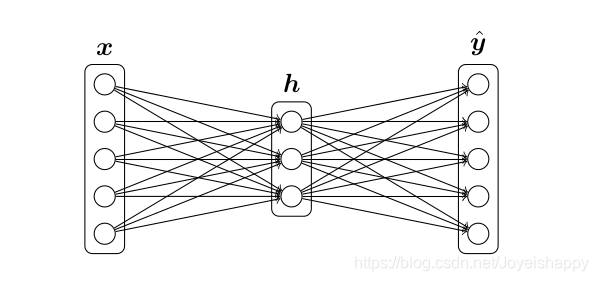
相关的两个前向传导的式子：

$h = sigmoid(xW_{1}+b_{1})$

$\hat{y}_{i} = softmax(hW_{2}+b_{2})$

这里假定输入向量是个行向量，sigmoid函数作用于其中的每个数，W和b是每层的weights权重和biases偏置。两层各两个。

可以看看这个推导，感觉对理解反向传播有帮助。

首先利用前向传播算出每层的值， $z_{_{i}} (i={1,2,3})$

$z_{1} = x$

$z_{2} = W_{1}x + b_{1}$

$z_{3} = W_{2}h+b_{2}$

反向求导：

输出是softmax函数，为使其损失函数（交叉熵函数CE）最小，对损失函数求梯度（对变量X求导）。(这里就会感受到反向传播的意思了...)

$\frac{\partial CE}{\partial z_{3}} = \delta _{3} = \hat{y} -y$ 先对 z3 求导，

$\frac{\partial CE}{\partial h}= \delta _{2} = \delta _{3}W_{2}^{T}$ z3里是不是有个变量h，变量h为系数矩阵W? 对，再对hW求导，

$\frac{\partial CE}{\partial z_{2}} = \delta _{1} = \delta _{2}\cdot \sigma '(z_{2})$ 然后！对h求导，也就是z2，后面那个sigma就是sigmoid求导嘛，前面有的。

$\frac{\partial CE}{\partial x} = \delta _{1}\frac{\partial z_{2}}{\partial x}=\delta _{1}W_{1}^{T}$ 终于目标函数看到x了，求导！即成。你看，这么一步一步反向传导，从后往前求出了我们想要的梯度了。

这个我是这么理解的，其实也是一个链式求导。一步一步对目标函数求导。

(d) 算参数有多少... 输入Dx维，输出Dy维，隐藏单元为H

$nW_{1} = D_{x} \times H&\\ nb_{1}= H &\\ nW_{2} =H \times D_{x} &\\ nb_{2}= D_{y}&\\ SUM_N = ( D_{x} +1)\times H + (H+1) \times D_{y}$

(e) 完成q2 sigmoid.py

这个简单。

import numpy as np

def sigmoid(x):
    """
    Compute the sigmoid function for the input here.

    Arguments:
    x -- A scalar or numpy array.

    Return:
    s -- sigmoid(x)
    """

    ### YOUR CODE HERE
    # raise NotImplementedError
    s = 1.0 / (np.exp(-x) + 1) 

    ### END YOUR CODE

    return s


def sigmoid_grad(s):
    """
    Compute the gradient for the sigmoid function here. Note that
    for this implementation, the input s should be the sigmoid
    function value of your original input x.

    Arguments:
    s -- A scalar or numpy array.

    Return:
    ds -- Your computed gradient.
    """

    #sigmoid函数求导： f'(x)= f(x)[1-f(x)] 


    ### YOUR CODE HERE
    # raise NotImplementedError

    ### END YOUR CODE
    ds =  s* (1 - s)

    return ds


def test_sigmoid_basic():
    """
    Some simple tests to get you started.
    Warning: these are not exhaustive.
    """
    print "Running basic tests..."
    x = np.array([[1, 2], [-1, -2]])
    f = sigmoid(x)
    g = sigmoid_grad(f)
    print f
    f_ans = np.array([
        [0.73105858, 0.88079708],
        [0.26894142, 0.11920292]])
    assert np.allclose(f, f_ans, rtol=1e-05, atol=1e-06)
    print g
    g_ans = np.array([
        [0.19661193, 0.10499359],
        [0.19661193, 0.10499359]])
    assert np.allclose(g, g_ans, rtol=1e-05, atol=1e-06)
    print "You should verify these results by hand!\n"


if __name__ == "__main__":
    test_sigmoid_basic()

(f)完成q2 gradcheck.py

这是个梯度检查的函数

代码里面有详细的注释，感觉说很多很罗嗦，凑合看吧，万一以后不明白了呢...

#coding:utf-8

import numpy as np
import random


# First implement a gradient checker by filling in the following functions
def gradcheck_naive(f, x):
    """ Gradient check for a function f.

    Arguments:
    f -- a function that takes a single argument and outputs the
         cost and its gradients
    x -- the point (numpy array) to check the gradient at
    """
    # 随机数的初始化
    rndstate = random.getstate()
    random.setstate(rndstate)

    # fx函数值，grad函数的导数值
    fx, grad = f(x) # Evaluate function value at original point
    # 这是一个很小的数h，目的呢，是根据导数定义，在x的领域，那领域呢，就是x左右很小的一部分包括x，这是数学上的定义了。
    # (f(x+h) - f(x-h）)/ 2h:这个公式呢，就是fx在X这一点的导数定义了。
    # 后面就是用这个公式来求导数的，然后和我们已知的根据法则公式得到导数 两个对比;
    # 就可以知道我们定义求的导数是否正确;
    h = 1e-4        # Do not change this!

    # Iterate over all indexes ix in x to check the gradient.
    # numpy array自带的迭代器，multi_index：多重索引[输出：就是数组索引号（0,0）（0,1）等]; readwrite：对x有可读可写的权限;iternext()：控制下一次迭代，如果没有这个控制下一次，就一直在一个索引值上操作;挺好用
    it = np.nditer(x, flags=['multi_index'], op_flags=['readwrite'])
    #判断有没有到结尾
    while not it.finished:
        # 数组索引值赋值
        ix = it.multi_index
        # Try modifying x[ix] with h defined above to compute numerical
        # gradients (numgrad).

        # Use the centered difference of the gradient.
        # It has smaller asymptotic error than forward / backward difference
        # methods. If you are curious, check out here:
        # https://math.stackexchange.com/questions/2326181/when-to-use-forward-or-central-difference-approximations

        # Make sure you call random.setstate(rndstate)
        # before calling f(x) each time. This will make it possible
        # to test cost functions with built in randomness later.

        ### YOUR CODE HERE:
        # 这里呢，主要运用的就是根据导数定义来求导数，

        x[ix] += h
        # 这个呢，其实我也没太明白，是一个随机数的状态设置？ 注释了这里，输出是一样的。提示说是为了以后随机测试 cost损失函数，可能后面有用吧。
        random.setstate(rndstate)
        # 取到函数值
        new_f1 = f(x)[0]

        #刚加了一个h
        x[ix] -= 2 * h
        random.setstate(rndstate)
        new_f2 = f(x)[0]

        # 这里呢 我们根据定义求得导数就出来了
        numgrad = (new_f1 - new_f2) / (2 * h)

        # raise NotImplementedError 



        ### END YOUR CODE

        # Compare gradients
        # 对比

        reldiff = abs(numgrad - grad[ix]) / max(1, abs(numgrad), abs(grad[ix]))
        # 定义求得导数是无限接近真实导数的，两者之间有差异，但是很小，这里用1e-5衡量
        if reldiff > 1e-5:
            print "Gradient check failed."
            print "First gradient error found at index %s" % str(ix)
            print "Your gradient: %f \t Numerical gradient: %f" % (
                grad[ix], numgrad)
            return

        # 去到下一个索引位置
        it.iternext() # Step to next dimension

    print "Gradient check passed!"


def sanity_check():
    """
    Some basic sanity checks.
    这里用x的平方测试
    """
    quad = lambda x: (np.sum(x ** 2), x * 2)

    print "Running sanity checks..."
    gradcheck_naive(quad, np.array(123.456))      # scalar test
    gradcheck_naive(quad, np.random.randn(3,))    # 1-D test
    gradcheck_naive(quad, np.random.randn(4,5))   # 2-D test
    print ""

if __name__ == "__main__":
    sanity_check()

(g)完成q2 q2 neural.py

这个作业就是对三层神经网络梯度求解的实现

# coding:utf-8
#!/usr/bin/env python

import numpy as np
import random

from q1_softmax import softmax
from q2_sigmoid import sigmoid, sigmoid_grad
from q2_gradcheck import gradcheck_naive


def forward_backward_prop(X, labels, params, dimensions):
    """
    Forward and backward propagation for a two-layer sigmoidal network

    Compute the forward propagation and for the cross entropy cost,
    the backward propagation for the gradients for all parameters.

    Notice the gradients computed here are different from the gradients in
    the assignment sheet: they are w.r.t. weights, not inputs.

    Arguments:
    X -- M x Dx matrix, where each row is a training example x.
    labels -- M x Dy matrix, where each row is a one-hot vector.
    params -- Model parameters, these are unpacked for you.
    dimensions -- A tuple of input dimension, number of hidden units
                  and output dimension
    """

    ### Unpack network parameters (do not modify)
    # 从params 取出所需要的参数;
    ofs = 0
    Dx, H, Dy = (dimensions[0], dimensions[1], dimensions[2])

    W1 = np.reshape(params[ofs:ofs+ Dx * H], (Dx, H))
    ofs += Dx * H
    b1 = np.reshape(params[ofs:ofs + H], (1, H))
    ofs += H
    W2 = np.reshape(params[ofs:ofs + H * Dy], (H, Dy))
    ofs += H * Dy
    b2 = np.reshape(params[ofs:ofs + Dy], (1, Dy))

    # Note: compute cost based on `sum` not `mean`.
    ### YOUR CODE HERE: forward propagation
    h = sigmoid(np.dot(X, W1) + b1)
    hat_y = softmax(np.dot(h, W2)  + b2)
    # raise NotImplementedError
    ### END YOUR CODE


    ### YOUR CODE HERE: backward propagation
    # raise NotImplementedError

    # 交叉熵损失函数值，因为真实数据是1, 所以没有写出来...
    cost = np.sum(-np.log(hat_y[labels==1])) / X.shape[0]

    #对z3求导
    d3 = (hat_y - labels) / X.shape[0]

    #z3那个式子
    gradW2 = np.dot(h.T, d3)
    gradb2 = np.sum(d3, 0, keepdims=True)
    

    #z2式子
    dh = np.dot(d3, W2.T)
    grad_h = sigmoid_grad(h) * dh

    gradW1 = np.dot(X.T,grad_h)
    gradb1 = np.sum(grad_h,0)

    ### END YOUR CODE

    ### Stack gradients (do not modify)
    # 把所有梯度值都连接在一起
    grad = np.concatenate((gradW1.flatten(), gradb1.flatten(),
        gradW2.flatten(), gradb2.flatten()))

    return cost, grad

结束！