


 这篇博客详细介绍了前端作业FE-HW1的内容,包括两个问题。Problem 1涉及统计分析、直方图绘制、行业统计以及变量转换。Problem 2涵盖了新变量生成、分组统计、缺失值检查、离群值处理和箱形图绘制。每个问题下又分为多个子任务,展示了数据处理的不同方面。
FE-HW1
文章目录
Problem 1
sysuse nlsw88.dta, clear //调入第一问的数据
1-(1)
1-(1) 统计age grade wage hours ttl_exp tenure的平均值、标准差、中位数、最小值和最大值并输出为Excel 表格可以接受的格式
			logout, save("$Out\Table01") excel replace: ///
				tabstat age grade wage hours ttl_exp tenure,      ///
				stat(mean sd p50 min max) format(%7.2f) column(statistic)
		**    variable |      mean        sd       p50       min       max
		**-------------+--------------------------------------------------
		**         age |     39.15      3.06     39.00     34.00     46.00
		**       grade |     13.10      2.52     12.00      0.00     18.00
		**        wage |      7.77      5.76      6.27      1.00     40.75
		**       hours |     37.22     10.51     40.00      1.00     80.00
		**     ttl_exp |     12.53      4.61     13.13      0.12     28.88
		**      tenure |      5.98      5.51      3.83      0.00     25.92
		**----------------------------------------------------------------
		**
1-(2)
1-(2) 产生新变量
			gen age2 = age^2         	//生成新变量age2等于age的平方
			gen ln_wage = ln(wage)   	//生成新变量ln_wage等于wage的自然对数
			egen wage_mean = mean(wage) //生成新变量wage_mean来表示wage的均值
			gen dum = (wage>wage_mean)  //生产新逻辑变量dum
1-(3)
1-(3) 绘制 ttl_exp 变量的直方图和密度函数图
			histogram ttl_exp			//绘制 ttl_exp 变量的直方图
			graph export His_ttl.png

			kdensity ttl_exp			//绘制 ttl_exp 变量的密度函数图
			graph export Kendi_ttl.png

由图形观察可知,ttl_exp的样本总体是一个右侧拖一个尾巴是正偏态分布
1-(4)
1-(4) 对industry做如下统计
1-(4)-(1)
1-(4)-(1) 每个行业的观察值个数
			logout, save("$Out\1-(4)-1") excel replace: ///
				tab industry
		*                         tab industry
		*
		*               industry |      Freq.     Percent        Cum.
		*------------------------+-----------------------------------
		*  Ag/Forestry/Fisheries |         17        0.76        0.76
		*                 Mining |          4        0.18        0.94
		*           Construction |         29        1.30        2.24
		*          Manufacturing |        367       16.44       18.68
		* Transport/Comm/Utility |         90        4.03       22.72
		* Wholesale/Retail Trade |        333       14.92       37.63
		*Finance/Ins/Real Estate |        192        8.60       46.24
		*    Business/Repair Svc |         86        3.85       50.09
		*      Personal Services |         97        4.35       54.44
		*  Entertainment/Rec Svc |         17        0.76       55.20
		*  Professional Services |        824       36.92       92.11
		*  Public Administration |        176        7.89      100.00
		*------------------------+-----------------------------------
		*                  Total |      2,232      100.00
1-(4)-(2)
1-(4)-(2) 各个行业妇女的平均工资(wage)、平均工作时数(hours)和平均年龄(age)
			logout, save("$Out\1-(4)-2") excel replace: ///
				bysort industry: tabstat wage hours age, ///
				stat(mean)  			//分组统计
*-> industry = Ag/Forestry/Fisheries	  *-> industry = Mining

*   stats |    wage     hours       age   *   stats |   wage     hours    age
*---------+------------------------------ *---------+---------------------------
*    mean |  5.621121  34.47059  39.94118 *    mean |  15.34959   40     37.25
*---------------------------------------- *-------------------------------------
*-> industry = Construction				  *-> industry = Manufacturing

*   stats |    wage     hours      age    *   stats |   wage     hours    age
*---------+------------------------------ *---------+---------------------------
*    mean |  7.564934  35.65517  38.62069 *    mean | 7.501578 40.89373  38.9891
*---------------------------------------- *-------------------------------------
*-> industry = Transport/Comm/Utility	  *-> industry = Wholesale/Retail Trade

*   stats |    wage     hours      age    *   stats |   wage     hours    age
*---------+------------------------------ *---------+---------------------------
*    mean |  11.44335  39.85556  39.27778 *    mean | 6.125897 35.24699 39.28829
*---------------------------------------- *-------------------------------------
*-> industry = Finance/Ins/Real Estate	  *-> industry = Business/Repair Svc

*   stats |    wage     hours      age    *   stats |   wage     hours    age
*---------+------------------------------ *---------+---------------------------
*    mean |  9.843174  38.51563  38.82813 *    mean | 7.51579 33.15116  38.73256
*---------------------------------------- *-------------------------------------
*-> industry = Personal Services    	  *-> industry = Entertainment/Rec Svc

*   stats |    wage     hours      age    *   stats |   wage     hours    age
*---------+------------------------------ *---------+---------------------------
*    mean | 7.871186  36.71655  39.23908  *    mean | 6.724409 34.35294 40.11765
*---------------------------------------- *-------------------------------------
*-> industry = Professional Services	  *-> industry = Public Administration

*   stats |    wage     hours      age    *   stats |   wage     hours    age
*---------+------------------------------ *---------+---------------------------
*    mean |  7.871186  36.71655  39.23908 *    mean | 9.148407 38.54545 39.15909
*---------------------------------------- *-------------------------------------
*-> industry = .

*   stats |      wage     hours       age
*---------+------------------------------
*    mean |   5.13411        35  40.28571
*----------------------------------------
1-(4)-(3)
1-(4)-(3) 统计不同行业中白种人、黑种人和其他人种的比例
			logout, save("$Out\1-(4)-3") excel replace: ///
			tab industry race, col  	//分组统计频率
		*                      |               race
		*             industry |     white      black      other |     Total
		*----------------------+---------------------------------+----------
		*Ag/Forestry/Fisheries |        13          4          0 |        17
		*                      |      0.80       0.69       0.00 |      0.76
		*----------------------+---------------------------------+----------
		*               Mining |         4          0          0 |         4
		*                      |      0.25       0.00       0.00 |      0.18
		*----------------------+---------------------------------+----------
		*         Construction |        24          4          1 |        29
		*                      |      1.48       0.69       3.85 |      1.30
		*----------------------+---------------------------------+----------
		*        Manufacturing |       229        134          4 |       367
		*                      |     14.07      23.14      15.38 |     16.44
		*----------------------+---------------------------------+----------
		*Transport/Comm/Utilit |        62         27          1 |        90
		*                      |      3.81       4.66       3.85 |      4.03
		*----------------------+---------------------------------+----------
		*Wholesale/Retail Trad |       267         66          0 |       333
		*                      |     16.41      11.40       0.00 |     14.92
		*----------------------+---------------------------------+----------
		*Finance/Ins/Real Esta |       165         25          2 |       192
		*                      |     10.14       4.32       7.69 |      8.60
		*----------------------+---------------------------------+----------
		*  Business/Repair Svc |        64         20          2 |        86
		*                      |      3.93       3.45       7.69 |      3.85
		*----------------------+---------------------------------+----------
		*    Personal Services |        51         45          1 |        97
		*                      |      3.13       7.77       3.85 |      4.35
		*----------------------+---------------------------------+----------
		*Entertainment/Rec Svc |        14          3          0 |        17
		*                      |      0.86       0.52       0.00 |      0.76
		*----------------------+---------------------------------+----------
		*Professional Services |       616        197         11 |       824
		*                      |     37.86      34.02      42.31 |     36.92
		*----------------------+---------------------------------+----------
		*Public Administration |       118         54          4 |       176
		*                      |      7.25       9.33      15.38 |      7.89
		*----------------------+---------------------------------+----------
		*                Total |     1,627        579         26 |     2,232
		*                      |    100.00     100.00     100.00 |    100.00
1-(5)
1-(5) 为race变量做标签
			label define race 1 "白种人" 2 "黑种人" 3 "其它"
			label value race race		//将值签race赋给变量race
1-(6)
1-(6) 续别变量转类别变量
1-(6)-(1)
1-(6)-(1) 按规则产生新变量G_age
			gen G_age = 1
			replace G_age = 2 if(37<age)
			replace G_age = 3 if(42<age)
1-(6)-(2)
1-(6)-(2) 为G_age变量添加数字-文字对应表
			label define G_age 1 "37岁以下" 2 "38岁到42岁之间" 3 "43岁以上"
			label value G_age G_age		//将值签G_age赋给变量G_age
Problem 2
webuse "nhanes2f.dta", clear //调入第二问的数据
2-(1)
2-(1)根据要求生成新变量av_height
bysort race : egen av_height = mean(height)
2-(2)
2-(2)根据要求生成新变量sd_height
egen sd_height = std(height)
2-(3)
2-(3)先依次求出按各个变量分组的组态别数,可能的组合个数为三者之积
bysort sex : count //按sex分类计数
            *---------------------------------------------------------------
			*-> sex = Male
			*4,909
			*---------------------------------------------------------------
			*-> sex = Female
			*5,428
			//则按sex分类有2个组态别
bysort race : count //按race分类计数
            *---------------------------------------------------------------
			*-> race = White
			*  9,051
			*---------------------------------------------------------------
			*-> race = Black
			*  1,086
			*---------------------------------------------------------------
			*-> race = Other
			*  200
			//按race分类有3个组态别
bysort region : count //按region分类计数
			*-> region = NE
			*2,086
			*---------------------------------------------------------------
			*-> region = MW
			*2,773
			*---------------------------------------------------------------
			*-> region = S
			*2,853
			*---------------------------------------------------------------
			*-> region = W
			*2,625
			//按region分类有4个组态别
			* 所以共有2*3*4=24个组态别,接下来输出每个组态别的个数
		logout, save("$Out\2-(3)") excel replace: ///
			bysort sex race region : count
			* bysort sex race region : count
			*---------------------------------------------------------------
			*-> sex = Male, race = White, region = NE
			*957
			*---------------------------------------------------------------
			*-> sex = Male, race = White, region = MW
			*1,170
			*---------------------------------------------------------------
			*-> sex = Male, race = White, region = S
			*1,076
			*---------------------------------------------------------------
			*-> sex = Male, race = White, region = W
			*1,103
			*---------------------------------------------------------------
			*-> sex = Male, race = Black, region = NE
			*51
			*---------------------------------------------------------------
			*-> sex = Male, race = Black, region = MW
			*133
			*---------------------------------------------------------------
			*-> sex = Male, race = Black, region = S
			*247
			*---------------------------------------------------------------
			*-> sex = Male, race = Black, region = W
			*69
			*---------------------------------------------------------------
			*-> sex = Male, race = Other, region = NE
			*5
			*---------------------------------------------------------------
			*-> sex = Male, race = Other, region = MW
			*7
			*---------------------------------------------------------------
			*-> sex = Male, race = Other, region = S
			*9
			*---------------------------------------------------------------
			*-> sex = Male, race = Other, region = W
			*82
			*---------------------------------------------------------------
			*-> sex = Female, race = White, region = NE
			*1,012
			*---------------------------------------------------------------
			*-> sex = Female, race = White, region = MW
			*1,291
			*---------------------------------------------------------------
			*-> sex = Female, race = White, region = S
			*1,208
			*---------------------------------------------------------------
			*-> sex = Female, race = White, region = W
			*1,234
			*---------------------------------------------------------------
			*-> sex = Female, race = Black, region = NE
			*55
			*---------------------------------------------------------------
			*-> sex = Female, race = Black, region = MW
			*162
			*---------------------------------------------------------------
			*-> sex = Female, race = Black, region = S
			*301
			*---------------------------------------------------------------
			*-> sex = Female, race = Black, region = W
			*68
			*---------------------------------------------------------------
			*-> sex = Female, race = Other, region = NE
			*6
			*---------------------------------------------------------------
			*-> sex = Female, race = Other, region = MW
			*10
			*---------------------------------------------------------------
			*-> sex = Female, race = Other, region = S
			*12
			*---------------------------------------------------------------
			*-> sex = Female, race = Other, region = W
			*69
2-(4)
2-(4)首先查看各个变量缺漏值的个数
misstable sum tcresult tgresult hdresult corpuscl health sizplace
*       misstable sum tcresult tgresult hdresult corpuscl health sizplace
*                                                             Obs<.
*                                              +------------------------------
*             |                                | Unique
*    Variable |     Obs=.     Obs>.     Obs<.  | values        Min         Max
*-------------+--------------------------------+------------------------------
*    tgresult |     5,293               5,044  |    423         16        2238
*    hdresult |     1,629               8,708  |    108         15         187
*    corpuscl |        89              10,248  |    411       58.3       125.9
*      health |         2              10,335  |      5          1           5
*-----------------------------------------------------------------------------
		//其中tcresult因为没有缺漏值没有没有显示在Variable中
		//接下来删除缺漏值
		dropmiss tgresult hdresult corpuscl,obs force any
		//删除之后检查删除效果
		misstable sum tgresult hdresult corpuscl
			*       misstable sum tgresult hdresult corpuscl
			*(variables nonmissing or string)
2-(5)
2-(5)首先求出height的第25百分位和第75百分位,再计算四分位间距,最后得到上下界
tabstat height , stat(p25 p75)
			*	       tabstat height , stat(p25 p75)
			*
			*	variable  |     p25       p75
			*-------------+--------------------
			*	height    |   160.699   175.098
			*----------------------------------

			*第25百分位为160.699,第75百分位为175.098,所以四分位间距为14.399
			*上界为Q3+1.5*IQR=196.697,下界为Q1-1.5*IQR=139.101
2-(6)
2-(6)绘制height和weight的箱形图
graph box height
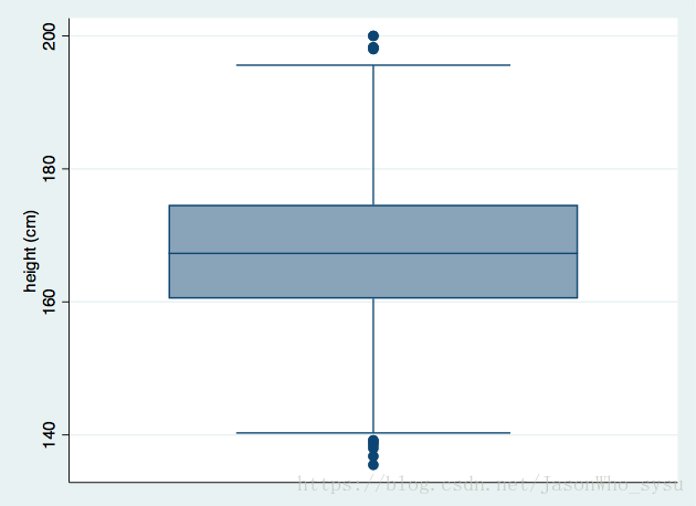
graph box weight
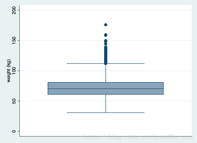
观察图形可知,身高有巨人和侏儒这样的离群值,而体重只有超重的离群值而没有超轻的离群值。
2-(7)
2-(7) 生成一个新变量height_w,对height进行缩尾处理
winsor2 height, suffix(_w) cuts(1 99)


 2505
2505

 被折叠的 条评论
为什么被折叠?
被折叠的 条评论
为什么被折叠?
 到【灌水乐园】发言


