


一、数据准备
1.遥感影像拼接
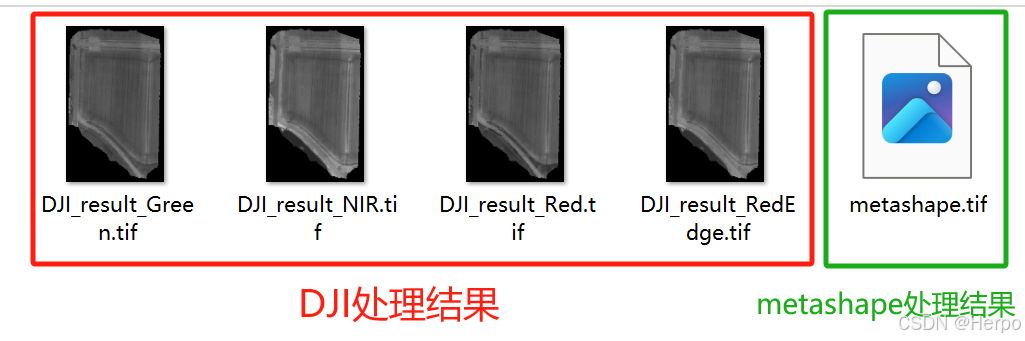
首先分别使用大疆智图和metashape对无人机多光谱影像进行拼接,metashape具体拼接流程参考在metashape中使用反射率标定板为多光谱数据校准,拼接结果如下,其中metashape导出的tif图存在4个波段,分别为R、G、B、RedEdge、NIR。
2.计算NDVI
使用拼接好的各波段数据计算NDVI,计算方法如下:
"""
使用metashape多波段图像,计算NDVI值
"""
import rasterio
import numpy as np
import matplotlib.pyplot as plt

# 读取多波段遥感图像
image_path = "metashape.tif"  # 替换为你的图像路径
with rasterio.open(image_path) as src:
    # 读取各个波段数据
    green_band = src.read(1)  # Band 1 - Green
    red_band = src.read(2)    # Band 2 - Red
    rededge_band = src.read(3) # Band 3 - RedEdge
    nir_band = src.read(4)    # Band 4 - NIR

    # 获取元数据用于保存结果
    crs = src.crs
    transform = src.transform
    width = src.width
    height = src.height

# 处理无效值:去除NaN和异常值(65535, -32767)
valid_mask = (nir_band != 65535) & (nir_band != -32767) & ~np.isnan(nir_band) & \
             (red_band != 65535) & (red_band != -32767) & ~np.isnan(red_band)

# 创建一个与原图像大小相同的全NaN数组
ndvi_result = np.full_like(nir_band, np.nan, dtype=np.float32)

# 应用掩码,计算有效区域的NDVI
ndvi_result[valid_mask] = (nir_band[valid_mask] - red_band[valid_mask]) / (nir_band[valid_mask] + red_band[valid_mask])

# 可视化NDVI结果
plt.imshow(ndvi_result, cmap='RdYlGn', vmin=np.nanmin(ndvi_result), vmax=1)
plt.colorbar()
plt.title('NDVI')
plt.show()

# 可选:保存NDVI结果为新的TIF文件
output_path = "metashape_ndvi_result.tif"
with rasterio.open(output_path, 'w', driver='GTiff',
                   count=1, dtype=ndvi_result.dtype,
                   crs=crs, transform=transform,
                   width=width, height=height) as dst:
    dst.write(ndvi_result, 1)
"""
计算DJI处理图像的NDVI
"""
import rasterio
import numpy as np
import matplotlib.pyplot as plt
# 读取红色波段和近红外波段的tif图像
red_band_path = "DJI_result_Red.tif" # 替换为红色波段图像路径
nir_band_path = "DJI_result_NIR.tif" # 替换为近红外波段图像路径
# 打开并读取红色波段图像
with rasterio.open(red_band_path) as red_src:
red_band = red_src.read(1) # 读取第一个波段的数据
# 打开并读取近红外波段图像
with rasterio.open(nir_band_path) as nir_src:
nir_band = nir_src.read(1) # 读取第一个波段的数据
# # 确保波段数据的形状一致
# assert red_band.shape == nir_band.shape, "红色波段和近红外波段的尺寸不匹配"
# 计算NDVI
ndvi = (nir_band - red_band) / (nir_band + red_band)
# 可选:保存NDVI结果为新的TIF文件
output_path = "DJI_ndvi_result.tif"
with rasterio.open(output_path, 'w', driver='GTiff',
count=1, dtype=ndvi.dtype,
crs=red_src.crs, transform=red_src.transform,
width=red_src.width, height=red_src.height) as dst:
dst.write(ndvi, 1)
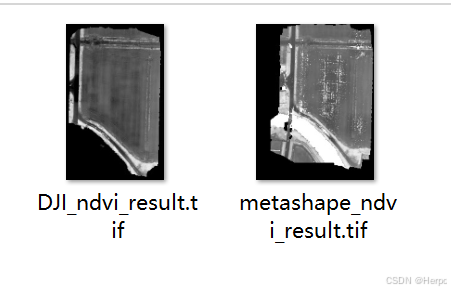
生成NDVI指数地图如下:
二、metashape与DJI拼图对比实验
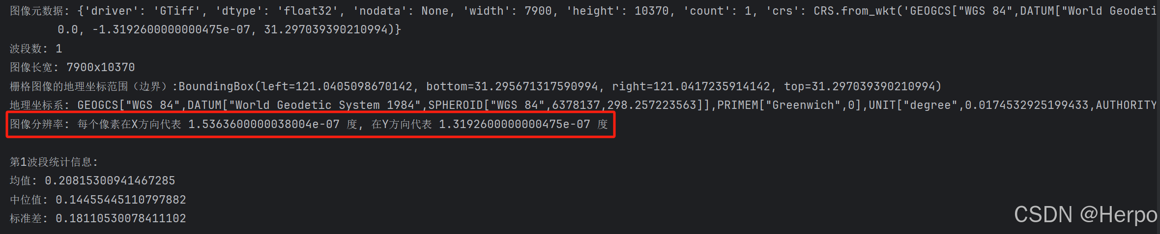
1.对比图像基本信息(tif_info.py)
- 图像的波段数、长宽、地理坐标系。
- 每个波段的均值、平均值、中位值、标准差。
- 输出图像分辨率(图中每个像素代表实际多长)
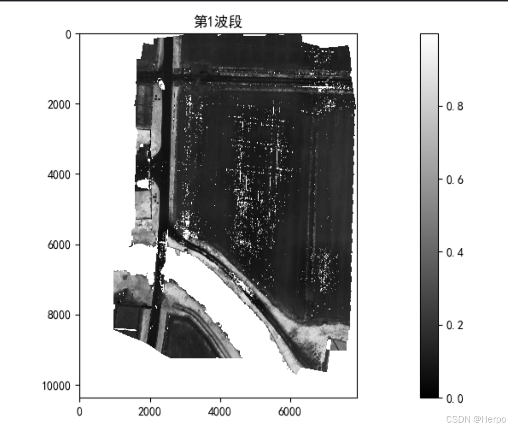
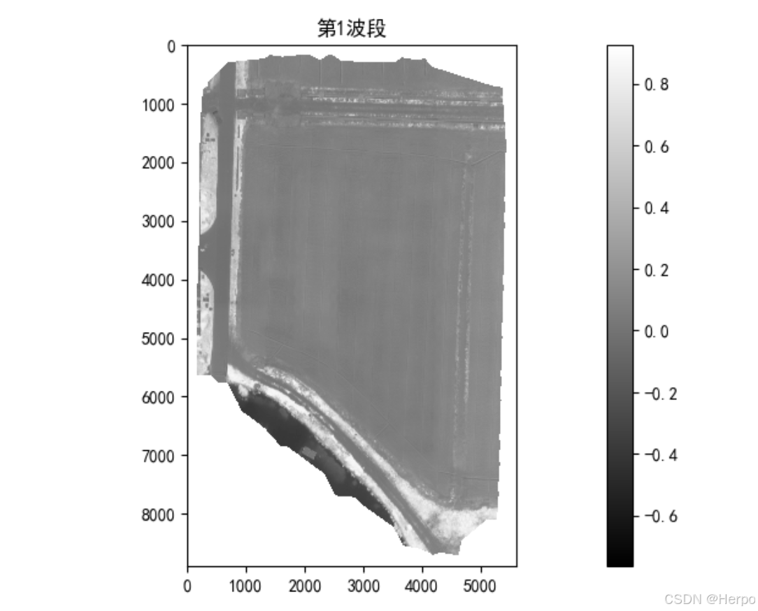
- 展示剔除空值及异常值的NDVI灰度图
- 图像在0到1之间的频率分布直方图
实现代码如下:
"""
本代码可输出以下信息:
1.图像的波段数、长宽、地理坐标系。
2.每个波段的均值、平均值、中位值、标准差。
3.输出图像分辨率(图中每个像素代表实际多长)
4.展示剔除空值及异常值的NDVI灰度图
5.图像在0到1之间的频率分布直方图
"""
import matplotlib.pyplot as plt
from matplotlib import rcParams
import rasterio
import numpy as np

# 设置字体为 SimHei (黑体)
rcParams['font.sans-serif'] = ['SimHei']  # 设置中文字体为黑体
rcParams['axes.unicode_minus'] = False  # 解决负号问题

# 读取多光谱遥感图像
image_path = "NDVI.tif"  # 替换为图像路径

with rasterio.open(image_path) as src:
    # 获取波段信息
    bands = src.read()  # 读取所有波段数据,返回一个NumPy数组
    band_count = bands.shape[0]  # 波段数目
    width = src.width  # 图像宽度
    height = src.height  # 图像高度
    bounds = src.bounds  # 栅格图像的地理坐标范围(边界)
    crs = src.crs  # 获取坐标参考系
    transform = src.transform  # 获取仿射变换矩阵(包含分辨率信息)

    # 获取图像的元数据
    metadata = src.meta
    print("图像元数据:", metadata)
    print(f"波段数: {band_count}")
    print(f"图像长宽: {width}x{height}")
    print(f"栅格图像的地理坐标范围(边界):{bounds}")
    print(f"地理坐标系: {crs}")

    # 计算图像分辨率(每个像素代表的实际长度)
    pixel_size_x = transform.a  # x 方向分辨率
    pixel_size_y = -transform.e  # y 方向分辨率
    print(f"图像分辨率: 每个像素在X方向代表 {pixel_size_x} 米, 在Y方向代表 {pixel_size_y} 米")

    # 设置绘图的行列数
    rows = int(np.ceil(band_count / 3))  # 每行显示3个波段(可根据需要调整)
    cols = min(band_count, 3)  # 每列最多显示3个波段

    # 创建子图
    plt.figure(figsize=(15, 5 * rows))  # 设置图形大小

    # 计算每个波段的统计信息并绘制图像
    for i in range(band_count):
        band = bands[i]  # 获取第i个波段数据

        # 删除值为65535, -32767和NaN的像素
        band = band[(band < 1) & (band != 65535) & (band != -32767) & ~np.isnan(band)]

        # 计算统计值
        mean = np.mean(band)  # 均值
        median = np.median(band)  # 中位值
        std = np.std(band)  # 标准差

        # 输出每个波段的统计信息
        print(f"\n第{i + 1}波段统计信息:")
        print(f"均值: {mean}")
        print(f"中位值: {median}")
        print(f"标准差: {std}")

        # 绘制图像
        plt.subplot(rows, cols, i + 1)  # 创建子图
        plt.imshow(bands[i], cmap='gray', vmin=np.min(band), vmax=np.max(band))  # 根据波段的最小值和最大值进行缩放
        plt.colorbar()
        plt.title(f'第{i + 1}波段')

    plt.tight_layout()  # 调整子图间距
    plt.show()

    # 绘制图像全体像素的频率分布直方图
    all_pixels = bands.flatten()  # 将所有波段的像素展开成一维数组
    all_pixels = all_pixels[(all_pixels < 1) & (all_pixels != 65535) & (all_pixels != -32767) & ~np.isnan(all_pixels)]  # 删除无效像素

    # 计算频率分布
    plt.figure(figsize=(10, 6))
    plt.hist(all_pixels, bins=50, color='gray', edgecolor='black', alpha=0.7)
    plt.title('所有像素值的频率分布')
    plt.xlabel('像素值')
    plt.ylabel('像素频率')
    plt.grid(True)
    plt.show()
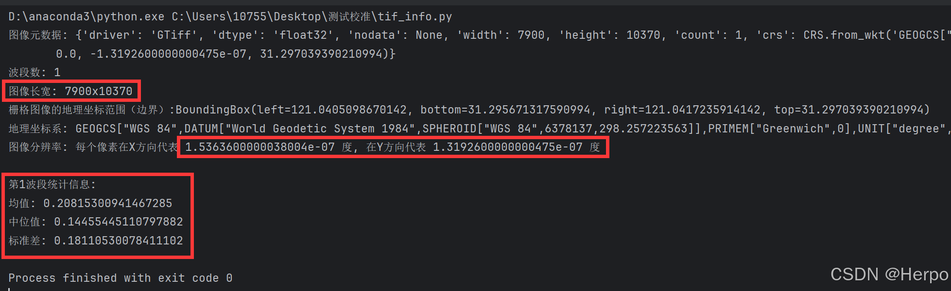
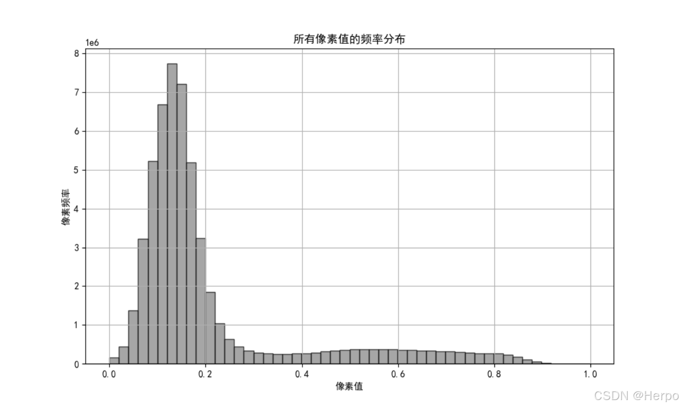
metashape_ndvi_result.tif输出结果如下:

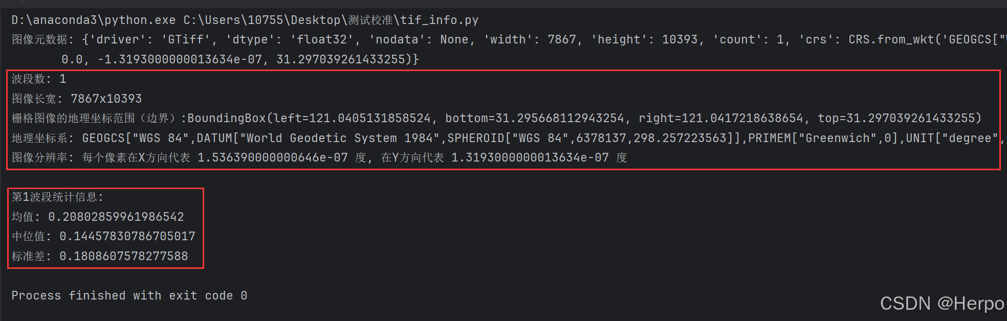
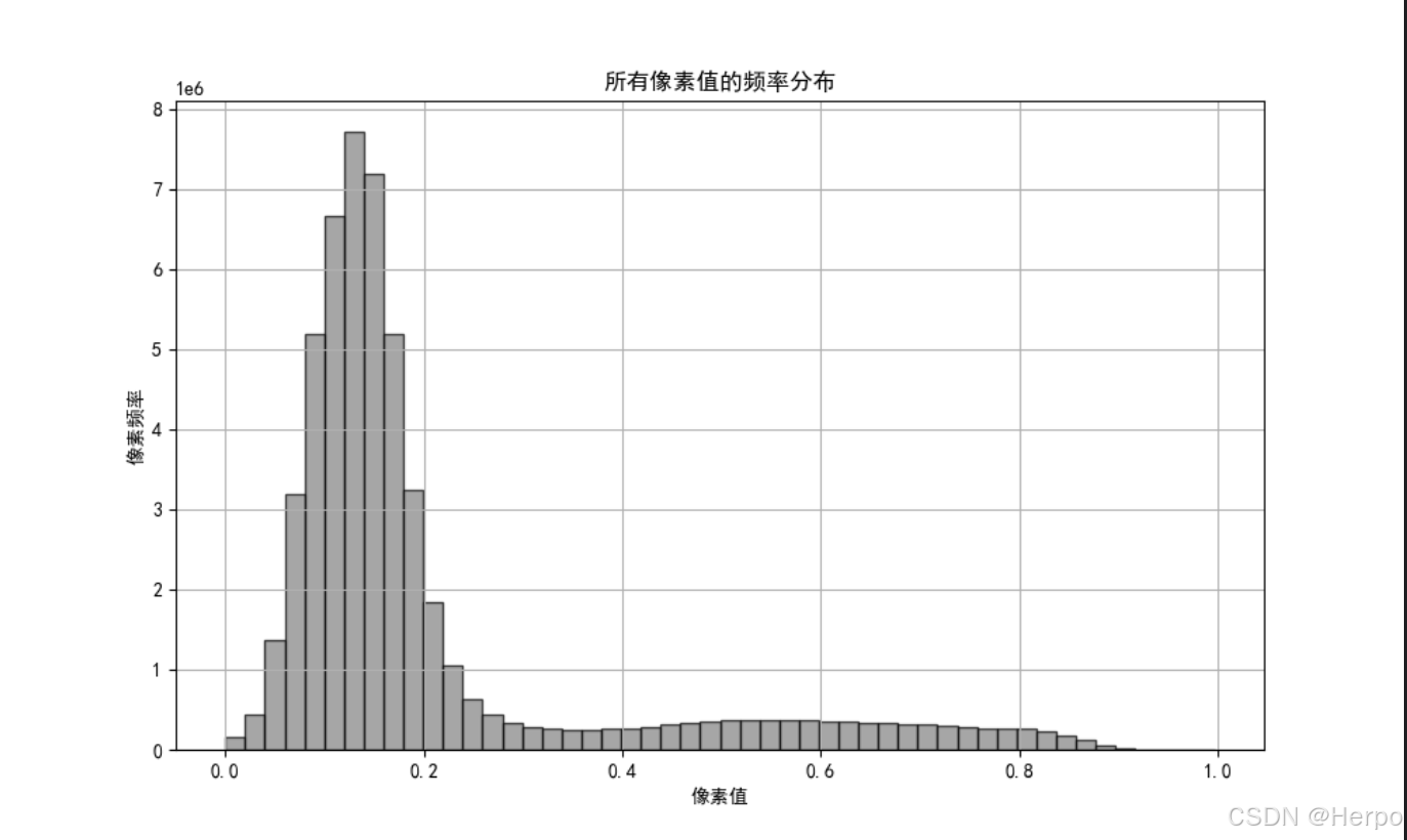
DJI_ndvi_result.tif输出结果如下:
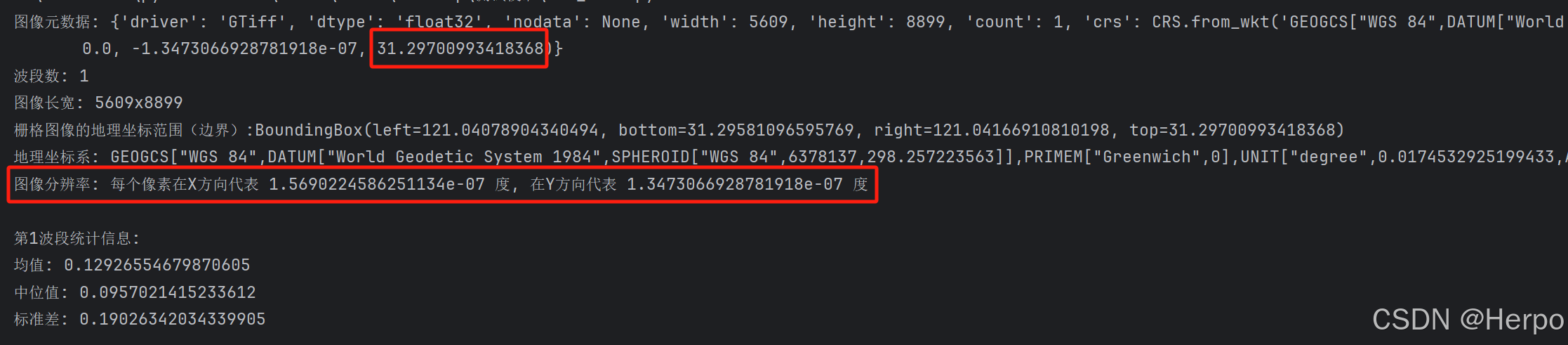
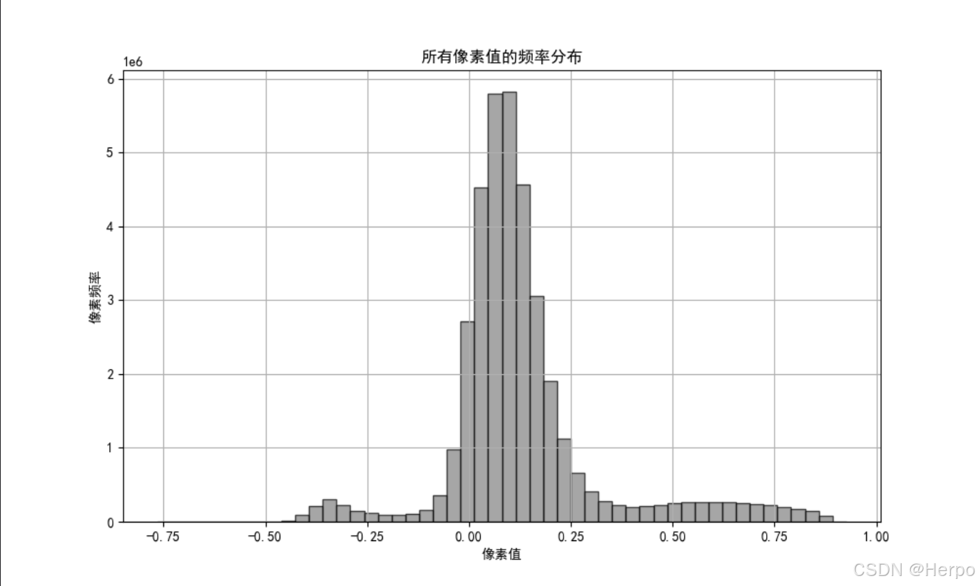
如图所示,注意红框内1.5363600000038004e-07的单位不是米,而是经纬度的1度,换算后每个像素代表的实际长度大概为0.15米。同时可以观察到频率分布在0到1之间较为相似。
2.对比相同坐标点下的指数取值(contrast.py)
思路如下:
- 在DJI_ndvi_result.tif图像中随机选择100个有效的地理坐标。
- 提取这些坐标点对应的像素值。
- 对metashape_ndvi_result.tif图像做同样的操作,确保使用相同的坐标。
- 筛选点的值需要在0到1之间,超出范围的点重新随机选择
- 对比提取的像素值,并做图展示差异情况
实现代码如下:
"""
对比DJI拼图与metashape拼图之间的差异
1.在一张TIFF图像中随机选择100个有效的地理坐标。
2.提取这些坐标点对应的像素值。
3.对另一张TIFF图像做同样的操作,确保使用相同的坐标。
4.对比提取的像素值
5.筛选点的值需要在0到1之间,超出范围的点重新随机选择
"""
import rasterio
import numpy as np
import random
import matplotlib.pyplot as plt
# 读取tif文件并提取坐标
def get_random_coordinates(raster_file, num_points):
with rasterio.open(raster_file) as src:
# 获取栅格的地理边界范围
bounds = src.bounds
print(f"栅格图像的地理坐标范围(边界):{bounds}")
random_coords = []
pixel_coords = []
while len(random_coords) < num_points:
# 随机生成坐标
x = random.uniform(bounds[0], bounds[2]) # 在左和右边界之间随机生成x坐标
y = random.uniform(bounds[1], bounds[3]) # 在下和上边界之间随机生成y坐标
coord = (x, y)
# 将地理坐标转换为像素坐标
pixel_coord = src.index(x, y)
# 提取像素值
value = src.read(1)[pixel_coord]
# 检查值是否在 0 到 1 之间,且不是 NaN
if not np.isnan(value) and 0 < value < 1:
random_coords.append(coord)
pixel_coords.append(pixel_coord)
print(f"筛选后的随机坐标:{random_coords}")
return random_coords, pixel_coords
# 提取指定坐标点的值
def extract_values(raster_file, pixel_coords):
with rasterio.open(raster_file) as src:
# 筛除空值
data = src.read(1) # 读取第一波段的数据
# 用0替换NaN值(你可以根据需要选择其他值)
data[np.isnan(data)] = 0
data[data > 1] = 0
data[data < 0] = 0
values = [data[x, y] for x, y in pixel_coords]
return values
# 对比两张tif图像在相同坐标点的值
def compare_rasters(raster_file_1, raster_file_2, num_points):
# 获取随机坐标和像素坐标
random_coords, pixel_coords = get_random_coordinates(raster_file_1, num_points)
# 提取两张图像中相同坐标点的像素值
values_1 = extract_values(raster_file_1, pixel_coords)
values_2 = extract_values(raster_file_2, pixel_coords)
# 计算值的差异
differences = np.array(values_1) - np.array(values_2)
# 输出对比结果
print("坐标对比结果:")
for i, (coord, v1, v2, diff) in enumerate(zip(random_coords, values_1, values_2, differences)):
print(
f"第 {i + 1} 个点: 坐标 {coord}, 栅格1中的值: {v1}, 栅格2中的值: {v2}, 差异: {diff}")
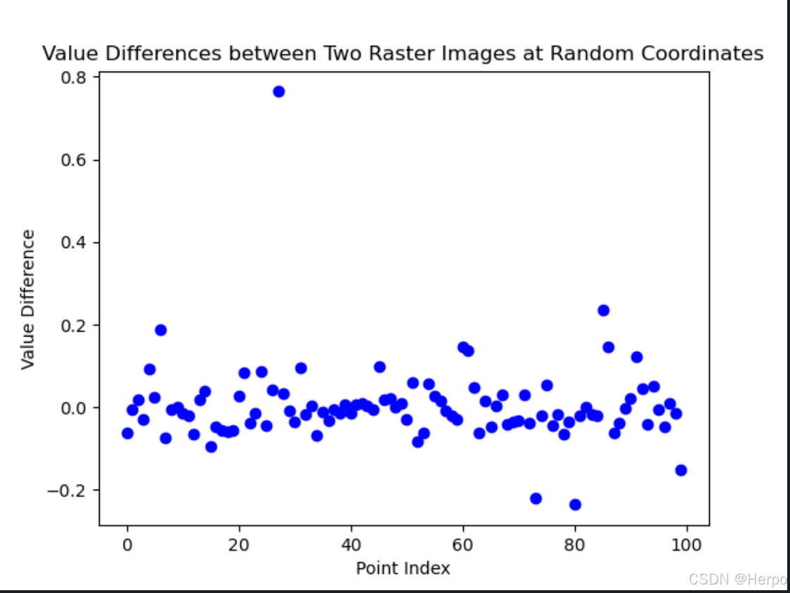
# 可视化差异
plt.scatter(range(num_points), differences, color='blue', label='Difference')
plt.xlabel('Point Index')
plt.ylabel('Value Difference')
plt.title('Value Differences between Two Raster Images at Random Coordinates')
plt.show()
if __name__ == "__main__":
# 调用示例
raster_file_1 = 'DJI_ndvi_result.tif'
raster_file_2 = 'metashape_ndvi_result.tif'
compare_rasters(raster_file_1, raster_file_2, num_points=100)
输出结果如下:
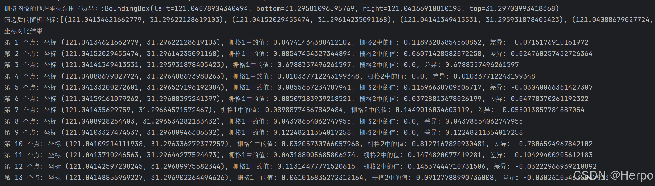
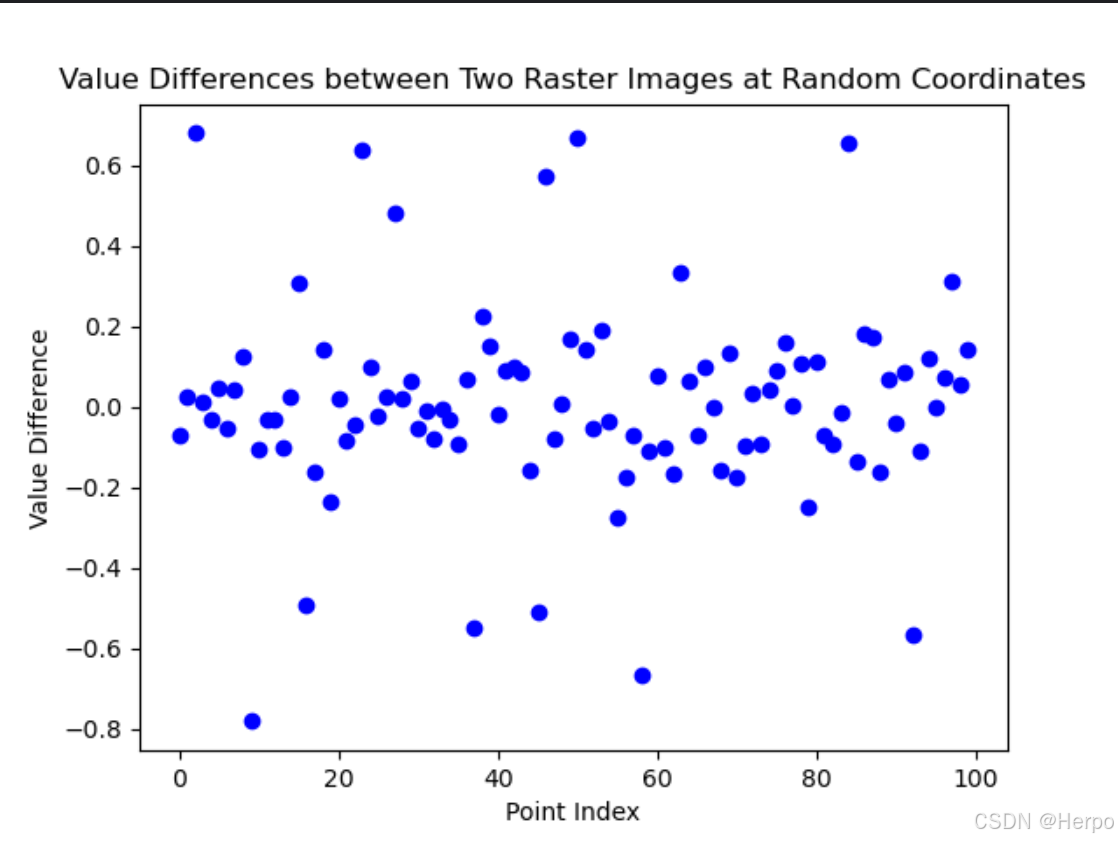
如图,DJI与matashape在相同坐标点下的NDVI值集中在[-0.4,0.4]范围内,差异相对较大。
3.各采样点10×10窗口均值对比(contrast1.py)
为了规避拼图偏移差异,选择采样点周围10×10窗口内的所有值取平均后再进行对比,代码如下:
"""
测试两张tif图中 采样点10×10窗口的均值差异,并进行相关性分析
"""
import rasterio
import numpy as np
import random
import matplotlib.pyplot as plt
# 读取tif文件并提取坐标
def get_random_coordinates(raster_file, num_points, window_size=5):
with rasterio.open(raster_file) as src:
# 获取栅格的地理边界范围
bounds = src.bounds
print(f"栅格图像的地理坐标范围(边界):{bounds}")
random_coords = []
pixel_coords = []
while len(random_coords) < num_points:
# 随机生成坐标
x = random.uniform(bounds[0], bounds[2]) # 在左和右边界之间随机生成x坐标
y = random.uniform(bounds[1], bounds[3]) # 在下和上边界之间随机生成y坐标
coord = (x, y)
# 将地理坐标转换为像素坐标
pixel_coord = src.index(x, y)
# 确保不会超出栅格的边界
min_x = max(pixel_coord[0] - window_size // 2, 0)
max_x = min(pixel_coord[0] + window_size // 2, src.width)
min_y = max(pixel_coord[1] - window_size // 2, 0)
max_y = min(pixel_coord[1] + window_size // 2, src.height)
# 生成窗口区域的坐标
window = (min_x, max_x, min_y, max_y)
random_coords.append(coord)
pixel_coords.append(window)
print(f"筛选后的随机坐标:{random_coords}")
return random_coords, pixel_coords
# 提取指定坐标点周围窗口区域的均值
def extract_values(raster_file, pixel_coords):
with rasterio.open(raster_file) as src:
# 读取栅格数据
data = src.read(1) # 读取第一波段的数据
# 用0替换NaN值(你可以根据需要选择其他值)
data[np.isnan(data)] = 0
data[data > 1] = 0
data[data < 0] = 0
mean_values = []
for window in pixel_coords:
min_x, max_x, min_y, max_y = window
# 提取窗口区域的像素值
window_data = data[min_y:max_y, min_x:max_x]
# 计算窗口区域的均值
mean_value = np.nanmean(window_data) # 使用np.nanmean避免NaN影响
mean_values.append(mean_value)
return mean_values
# 对比两张tif图像在相同坐标点的值
def compare_rasters(raster_file_1, raster_file_2, num_points):
# 获取随机坐标和像素坐标
random_coords, pixel_coords = get_random_coordinates(raster_file_1, num_points)
# 提取两张图像中相同坐标点的窗口均值
values_1 = extract_values(raster_file_1, pixel_coords)
values_2 = extract_values(raster_file_2, pixel_coords)
# 计算值的差异
differences = np.array(values_1) - np.array(values_2)
# 输出对比结果
print("坐标对比结果:")
for i, (coord, v1, v2, diff) in enumerate(zip(random_coords, values_1, values_2, differences)):
print(
f"第 {i + 1} 个点: 坐标 {coord}, 栅格1中的均值: {v1}, 栅格2中的均值: {v2}, 差异: {diff}")
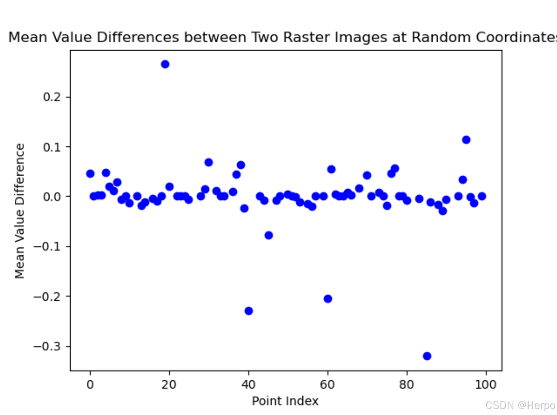
# 可视化差异
plt.scatter(range(num_points), differences, color='blue', label='Difference')
plt.xlabel('Point Index')
plt.ylabel('Mean Value Difference')
plt.title('Mean Value Differences between Two Raster Images at Random Coordinates')
plt.show()
if __name__ == "__main__":
# 调用示例
raster_file_1 = 'DJI_ndvi_result.tif'
raster_file_2 = 'metashape_ndvi_result.tif'
compare_rasters(raster_file_1, raster_file_2, num_points=100)输出结果如下:
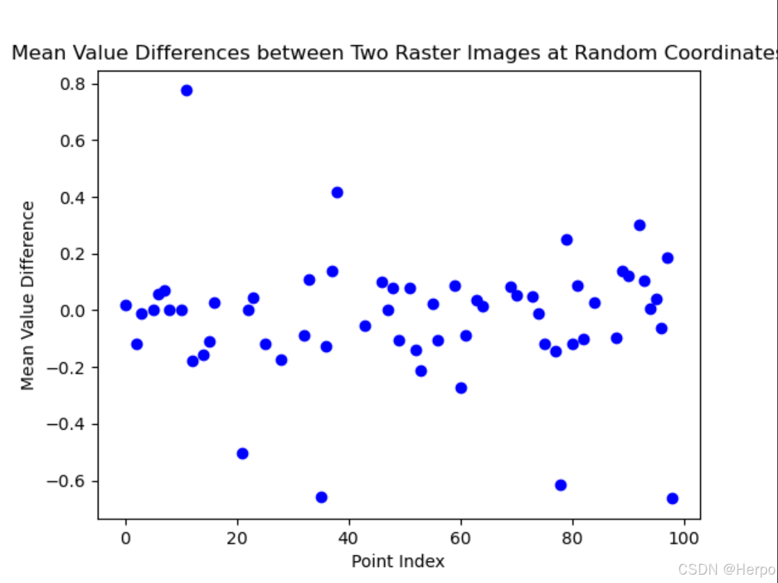
如图所示,计算10×10窗格的均值后,结果差异没有明显提升。
4.相关性分析(contrast2.py)
基于contrast.py,增加了对比相应坐标点相关性的功能。
"""
基于contrast.py,增加了对比相应坐标点相关性的功能
"""
import rasterio
import numpy as np
import random
import matplotlib.pyplot as plt
from scipy.stats import pearsonr # 导入皮尔逊相关系数计算函数
# 读取tif文件并提取坐标
def get_random_coordinates(raster_file, num_points):
with rasterio.open(raster_file) as src:
# 获取栅格的地理边界范围
bounds = src.bounds
print(f"栅格图像的地理坐标范围(边界):{bounds}")
random_coords = []
pixel_coords = []
while len(random_coords) < num_points:
# 随机生成坐标
x = random.uniform(bounds[0], bounds[2]) # 在左和右边界之间随机生成x坐标
y = random.uniform(bounds[1], bounds[3]) # 在下和上边界之间随机生成y坐标
coord = (x, y)
# 将地理坐标转换为像素坐标
pixel_coord = src.index(x, y)
# 提取像素值
value = src.read(1)[pixel_coord]
# 检查值是否在 0 到 1 之间,且不是 NaN
if not np.isnan(value) and 0 < value < 1:
random_coords.append(coord)
pixel_coords.append(pixel_coord)
print(f"筛选后的随机坐标:{random_coords}")
return random_coords, pixel_coords
# 提取指定坐标点的值,并过滤掉值为0、NaN和inf的点
def extract_values(raster_file, pixel_coords):
with rasterio.open(raster_file) as src:
# 读取第一波段的数据
data = src.read(1)
# 提取像素值,并过滤掉值为0、NaN和inf的点
values = []
valid_pixel_coords = []
for x, y in pixel_coords:
value = data[x, y]
if value != 0 and not np.isnan(value) and not np.isinf(value): # 过滤掉值为0、NaN和inf的点
values.append(value)
valid_pixel_coords.append((x, y))
return values, valid_pixel_coords
# 对比两张tif图像在相同坐标点的值,并计算相关性
def compare_rasters(raster_file_1, raster_file_2, num_points):
# 获取随机坐标和像素坐标
random_coords, pixel_coords = get_random_coordinates(raster_file_1, num_points)
# 提取两张图像中相同坐标点的像素值,并过滤掉值为0、NaN和inf的点
values_1, valid_pixel_coords_1 = extract_values(raster_file_1, pixel_coords)
values_2, valid_pixel_coords_2 = extract_values(raster_file_2, valid_pixel_coords_1)
# 确保两张图像的有效坐标点完全一致
if len(values_1) != len(values_2):
print("警告:两张图像的有效坐标点数量不一致,可能是某些点在第二张图像中值为0、NaN或inf。")
# 取两张图像有效坐标点的交集
valid_indices = [i for i, (x1, y1) in enumerate(valid_pixel_coords_1)
if (x1, y1) in valid_pixel_coords_2]
values_1 = [values_1[i] for i in valid_indices]
values_2 = [values_2[valid_pixel_coords_2.index(valid_pixel_coords_1[i])] for i in valid_indices]
# 将值转换为NumPy数组
values_1 = np.array(values_1)
values_2 = np.array(values_2)
# 检查是否有足够的有效点
if len(values_1) == 0 or len(values_2) == 0:
print("没有足够的有效点来计算相关性。")
return
# 检查数组中是否包含NaN或inf
if np.any(np.isnan(values_1)) or np.any(np.isinf(values_1)) or np.any(np.isnan(values_2)) or np.any(np.isinf(values_2)):
print("警告:数组中包含NaN或inf值,无法计算皮尔逊相关系数。")
return
# 计算差值
differences = values_1 - values_2
# 过滤掉差值大于1的点
valid_indices = np.abs(differences) <= 0.35 # 差值在 [-0.35, 0.35] 范围内的点
values_1 = values_1[valid_indices]
values_2 = values_2[valid_indices]
differences = differences[valid_indices]
# 检查过滤后是否有足够的有效点
if len(values_1) == 0 or len(values_2) == 0:
print("没有足够的有效点来计算相关性(差值过滤后无有效点)。")
return
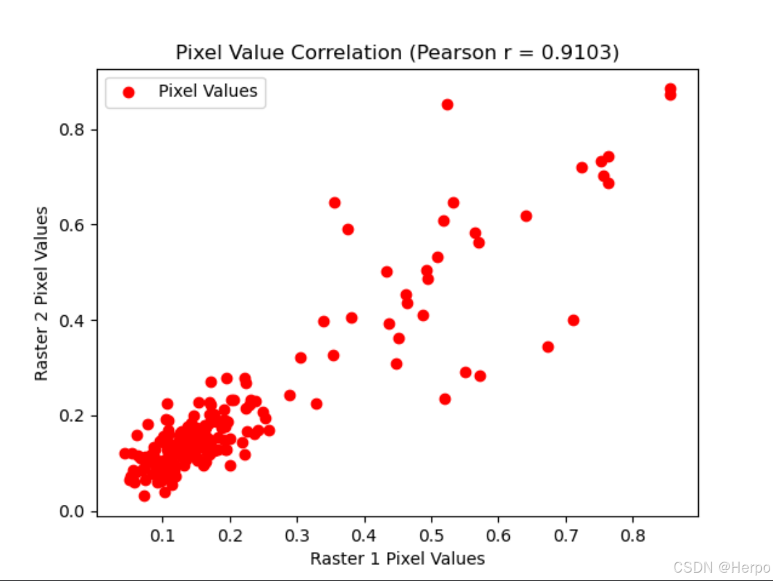
# 计算皮尔逊相关系数
correlation, _ = pearsonr(values_1, values_2)
print(f"两张图像的像素值皮尔逊相关系数: {correlation:.4f}")
# 输出对比结果
print("坐标对比结果:")
for i, (v1, v2, diff) in enumerate(zip(values_1, values_2, differences)):
print(
f"第 {i + 1} 个点: 栅格1中的值: {v1:.4f}, 栅格2中的值: {v2:.4f}, 差异: {diff:.4f}")
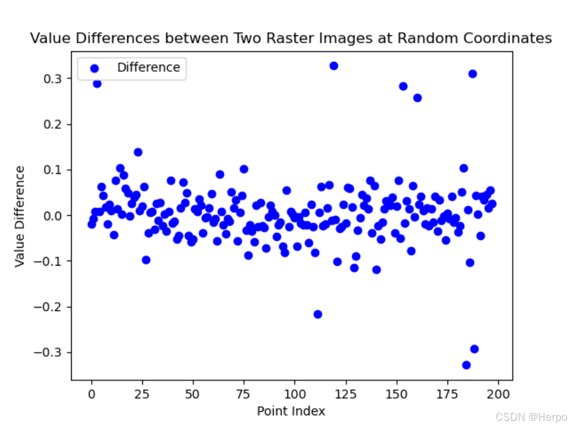
# 可视化差异
plt.scatter(range(len(differences)), differences, color='blue', label='Difference')
plt.xlabel('Point Index')
plt.ylabel('Value Difference')
plt.title('Value Differences between Two Raster Images at Random Coordinates')
plt.legend()
plt.show()
# 可视化相关性
plt.scatter(values_1, values_2, color='red', label='Pixel Values')
plt.xlabel('Raster 1 Pixel Values')
plt.ylabel('Raster 2 Pixel Values')
plt.title(f'Pixel Value Correlation (Pearson r = {correlation:.4f})')
plt.legend()
plt.show()
if __name__ == "__main__":
# 调用示例
raster_file_1 = 'DJI_ndvi_result.tif'
raster_file_2 = 'metashape_ndvi_result.tif'
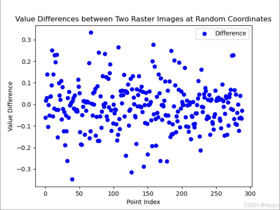
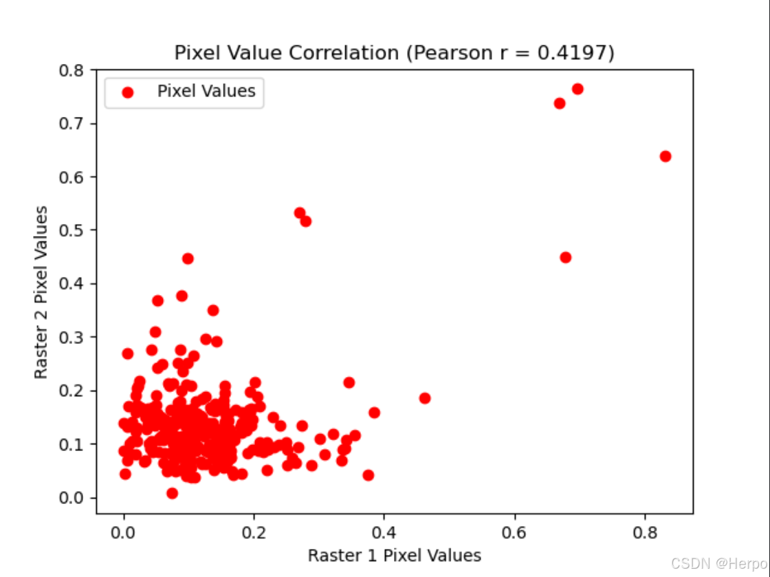
compare_rasters(raster_file_1, raster_file_2, num_points=500)结果如下:
三、对比matashape使用标定板及光学传感之间的差异实验
1.对比图像基本信息(tif_info.py)
代码同上
test1_ndvi.tif(使用校准板校准)结果如下:
test2_ndvi.tif(无校准板校准)结果如下:
对比发现,两张图像的基本信息几乎完全一致。
2.对比相同坐标点下的指数取值(contrast.py)
对比test1_ndvi.tif与test2_ndvi.tif,结果如下。相较于第二节的对比,test1与test2之间差异不大。
3.各采样点10×10窗口均值对比(contrast1.py)
计算均值后,两张tif图的差异进一步缩小。
4.相关性分析(contrast2.py)
结果如下,相关性很高。


 被折叠的 条评论
为什么被折叠?
被折叠的 条评论
为什么被折叠?
 到【灌水乐园】发言


