TensorFlow学习（7）tensorboard 网络结构

最新推荐文章于 2023-12-30 14:10:04 发布

换头像真麻烦

最新推荐文章于 2023-12-30 14:10:04 发布

阅读量298

点赞数

分类专栏：深度学习

本文链接：https://blog.youkuaiyun.com/HAIYUANBOY/article/details/89854122

版权

深度学习专栏收录该内容

13 篇文章

订阅专栏

本文介绍了如何使用TensorFlow中的TensorBoard进行网络结构的可视化，包括清理logs文件、命名空间的使用、代价函数和准确率的命名、观察loss变化、权重和偏置的histogram分布以及设置projector进行数据可视化。通过这些步骤，可以更清晰地理解和调试模型。

摘要生成于 C知道，由 DeepSeek-R1 满血版支持，前往体验 >

import tensorflow as tf
from tensorflow.examples.tutorials.mnist import input_data
# 载入数据集
mnist = input_data.read_data_sets('MNIST_data',one_hot=True)

# 不是一张张图片放入神经网络，定义一个批次，一次 100
batch_size = 100
# 计算一个有多少批次，整除
n_batch = mnist.train.num_examples // batch_size

# 命名空间
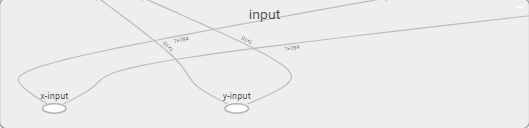
with tf.name_scope('input'):
    x = tf.placeholder(tf.float32, [None, 784],name='x-input')
    y = tf.placeholder(tf.float32, [None, 10],name='y-input')

# 创建一个简单的神经网络
W = tf.Variable(tf.zeros([784, 10]))
b = tf.Variable(tf.zeros([10]))
prediction = tf.nn.softmax(tf.matmul(x,W)+b)

# 二次代价函数
# loss = tf.reduce_mean(tf.square(y-prediction))
# 交叉熵代价函数配合 softmax 使用
# 因为 prediction 是通过 softmax 来的，它是类别概率数组，所以不能直接用普通的交叉熵函数
loss = tf.reduce_mean(tf.nn.softmax_cross_entropy_with_logits(labels=y, logits=prediction))

# 梯度下降法
train_step = tf.train.GradientDescentOptimizer(0.2).minimize(loss)

init = tf.global_variables_initializer()

# 结果存放在布尔型列表中
# tf.equal 相等返回 True，否则 False，argmax 比较 y 中哪个元素的值为 1，返回该元素下标
correct_predition = tf.equal(tf.argmax(y, 1), tf.argmax(prediction, 1))
# 求准确率
# tf.cast 将布尔型转换为32位浮点型，True -> 1.0，False -> 0.0，然后求平均值，如有 9 个 1,1 个 0，平均值为 0.9，准确率为 0.9
accuracy = tf.reduce_mean(tf.cast(correct_predition, tf.float32))

with tf.Session() as sess:
    sess.run(init)
    writer = tf.summary.FileWriter('logs/',sess.graph)
    # 循环 21 个周期，每个周期批次为 100，每个周期将所有图片都训练一次
    for epoch in range(1):
        for batch in range(n_batch):
            batch_xs, batch_ys = mnist.train.next_batch(batch_size)
            sess.run(train_step, feed_dict={x:batch_xs, y:batch_ys})
        #训练完一个周期看下准确率
        acc = sess.run(accuracy, feed_dict={x:mnist.test.images,y:mnist.test.labels})
        print('Iter ' + str(epoch) + ', Testing Accuracy' + str(acc))

增添这几行

# 命名空间
with tf.name_scope('input'):
    x = tf.placeholder(tf.float32, [None, 784],name='x-input')
    y = tf.placeholder(tf.float32, [None, 10],name='y-input')

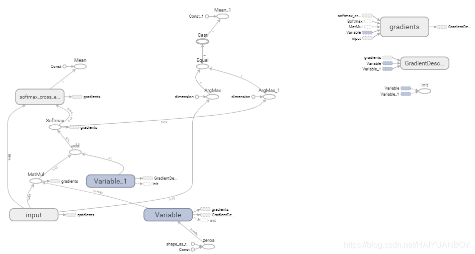
writer = tf.summary.FileWriter('logs/',sess.graph)

打开谷歌浏览器

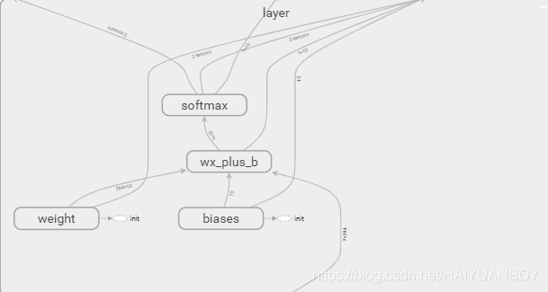
在隐藏层添加命名空间

with tf.name_scope('layer'):
    # 创建一个简单的神经网络
    with tf.name_scope('weight'):
        W = tf.Variable(tf.zeros([784, 10]),name='W')
    with tf.name_scope('biases'):
        b = tf.Variable(tf.zeros([10]))
    with tf.name_scope('wx_plus_b'):
        wx_plus_b = tf.matmul(x,W)+b
    with tf.name_scope('softmax'):
        prediction = tf.nn.softmax(wx_plus_b)

删除logs下生产的文件，重启notebook内核重新执行程序

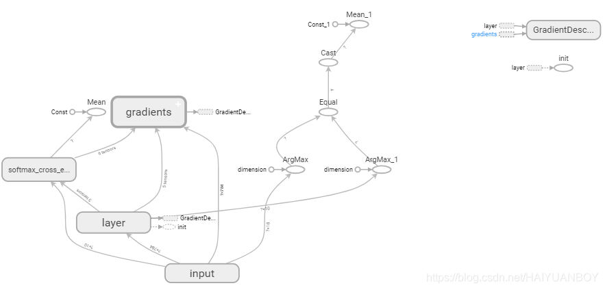
给代价函数和计算准确率添加命名空间

# 二次代价函数
# loss = tf.reduce_mean(tf.square(y-prediction))
with tf.name_scope('loss'):
    # 交叉熵代价函数配合 softmax 使用
    # 因为 prediction 是通过 softmax 来的，它是类别概率数组，所以不能直接用普通的交叉熵函数
    loss = tf.reduce_mean(tf.nn.softmax_cross_entropy_with_logits(labels=y, logits=prediction))
with tf.name_scope('train'):
    # 梯度下降法
    train_step = tf.train.GradientDescentOptimizer(0.2).minimize(loss)

init = tf.global_variables_initializer()

with tf.name_scope('count_accuracy'):
    with tf.name_scope('correct_predition'):
        # 结果存放在布尔型列表中
        # tf.equal 相等返回 True，否则 False，argmax 比较 y 中哪个元素的值为 1，返回该元素下标
        correct_predition = tf.equal(tf.argmax(y, 1), tf.argmax(prediction, 1))
    with tf.name_scope('accuracy'):
        # 求准确率
        # tf.cast 将布尔型转换为32位浮点型，True -> 1.0，False -> 0.0，然后求平均值，如有 9 个 1,1 个 0，平均值为 0.9，准确率为 0.9
        accuracy = tf.reduce_mean(tf.cast(correct_predition, tf.float32))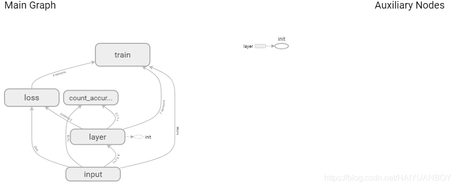

双击打开查看

完整程序

import tensorflow as tf
from tensorflow.examples.tutorials.mnist import input_data
# 载入数据集
mnist = input_data.read_data_sets('MNIST_data',one_hot=True)

# 不是一张张图片放入神经网络，定义一个批次，一次 100
batch_size = 100
# 计算一个有多少批次，整除
n_batch = mnist.train.num_examples // batch_size

# 命名空间
with tf.name_scope('input'):
    x = tf.placeholder(tf.float32, [None, 784],name='x-input')
    y = tf.placeholder(tf.float32, [None, 10],name='y-input')

with tf.name_scope('layer'):
    # 创建一个简单的神经网络
    with tf.name_scope('weight'):
        W = tf.Variable(tf.zeros([784, 10]),name='W')
    with tf.name_scope('biases'):
        b = tf.Variable(tf.zeros([10]))
    with tf.name_scope('wx_plus_b'):
        wx_plus_b = tf.matmul(x,W)+b
    with tf.name_scope('softmax'):
        prediction = tf.nn.softmax(wx_plus_b)

# 二次代价函数
# loss = tf.reduce_mean(tf.square(y-prediction))
with tf.name_scope('loss'):
    # 交叉熵代价函数配合 softmax 使用
    # 因为 prediction 是通过 softmax 来的，它是类别概率数组，所以不能直接用普通的交叉熵函数
    loss = tf.reduce_mean(tf.nn.softmax_cross_entropy_with_logits(labels=y, logits=prediction))
with tf.name_scope('train'):
    # 梯度下降法
    train_step = tf.train.GradientDescentOptimizer(0.2).minimize(loss)

init = tf.global_variables_initializer()

with tf.name_scope('count_accuracy'):
    with tf.name_scope('correct_predition'):
        # 结果存放在布尔型列表中
        # tf.equal 相等返回 True，否则 False，argmax 比较 y 中哪个元素的值为 1，返回该元素下标
        correct_predition = tf.equal(tf.argmax(y, 1), tf.argmax(prediction, 1))
    with tf.name_scope('accuracy'):
        # 求准确率
        # tf.cast 将布尔型转换为32位浮点型，True -> 1.0，False -> 0.0，然后求平均值，如有 9 个 1,1 个 0，平均值为 0.9，准确率为 0.9
        accuracy = tf.reduce_mean(tf.cast(correct_predition, tf.float32))

with tf.Session() as sess:
    sess.run(init)
    writer = tf.summary.FileWriter('logs/',sess.graph)
    # 循环 21 个周期，每个周期批次为 100，每个周期将所有图片都训练一次
    for epoch in range(1):
        for batch in range(n_batch):
            batch_xs, batch_ys = mnist.train.next_batch(batch_size)
            sess.run(train_step, feed_dict={x:batch_xs, y:batch_ys})
        #训练完一个周期看下准确率
        acc = sess.run(accuracy, feed_dict={x:mnist.test.images,y:mnist.test.labels})
        print('Iter ' + str(epoch) + ', Testing Accuracy' + str(acc))

删除logs下生产的文件，重启notebook内核重新执行程序

使用 tf.summary

with tf.name_scope('layer'):
    # 创建一个简单的神经网络
    with tf.name_scope('weight'):
        W = tf.Variable(tf.zeros([784, 10]),name='W')
        variable_summaries(W)
    with tf.name_scope('biases'):
        b = tf.Variable(tf.zeros([10]))
        variable_summaries(b)
    with tf.name_scope('wx_plus_b'):
        wx_plus_b = tf.matmul(x,W)+b
    with tf.name_scope('softmax'):
        prediction = tf.nn.softmax(wx_plus_b)


# 合并所有的 summary
merged = tf.summary.merge_all()

summary,_ = sess.run([merged,train_step], feed_dict={x:batch_xs, y:batch_ys})

writer.add_summary(summary, epoch)

具体代码如下

import tensorflow as tf
from tensorflow.examples.tutorials.mnist import input_data
# 载入数据集
mnist = input_data.read_data_sets('MNIST_data',one_hot=True)

# 不是一张张图片放入神经网络，定义一个批次，一次 100
batch_size = 100
# 计算一个有多少批次，整除
n_batch = mnist.train.num_examples // batch_size

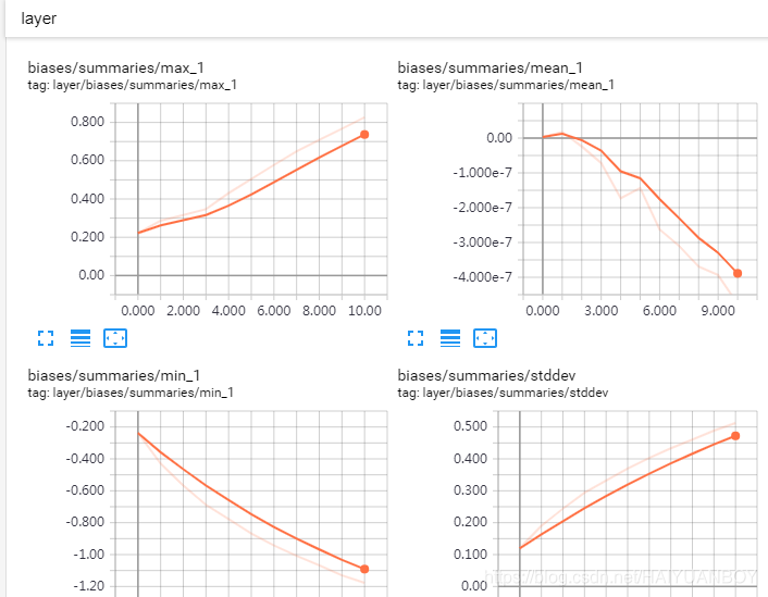
# 参数概要
def variable_summaries(var):
    with tf.name_scope('summaries'):
        mean = tf.reduce_mean(var)
        # scalar 记录这个值，且起名字
        tf.summary.scalar('mean', mean)
        with tf.name_scope('summaries'):
            stddev = tf.sqrt(tf.reduce_mean(tf.square(var - mean))) # 标准差
        tf.summary.scalar('stddev', stddev)
        tf.summary.scalar('max', tf.reduce_max(var))
        tf.summary.scalar('min', tf.reduce_min(var))
        tf.summary.histogram('histogram', var) # 直方图

# 命名空间
with tf.name_scope('input'):
    x = tf.placeholder(tf.float32, [None, 784],name='x-input')
    y = tf.placeholder(tf.float32, [None, 10],name='y-input')

with tf.name_scope('layer'):
    # 创建一个简单的神经网络
    with tf.name_scope('weight'):
        W = tf.Variable(tf.zeros([784, 10]),name='W')
        variable_summaries(W)
    with tf.name_scope('biases'):
        b = tf.Variable(tf.zeros([10]))
        variable_summaries(b)
    with tf.name_scope('wx_plus_b'):
        wx_plus_b = tf.matmul(x,W)+b
    with tf.name_scope('softmax'):
        prediction = tf.nn.softmax(wx_plus_b)

# 二次代价函数
# loss = tf.reduce_mean(tf.square(y-prediction))
with tf.name_scope('loss'):
    # 交叉熵代价函数配合 softmax 使用
    # 因为 prediction 是通过 softmax 来的，它是类别概率数组，所以不能直接用普通的交叉熵函数
    loss = tf.reduce_mean(tf.nn.softmax_cross_entropy_with_logits(labels=y, logits=prediction))
    # loss 只有一个值，没必要调用 variable_summaries 函数
    tf.summary.scalar('loss', loss)
with tf.name_scope('train'):
    # 梯度下降法
    train_step = tf.train.GradientDescentOptimizer(0.2).minimize(loss)

init = tf.global_variables_initializer()

with tf.name_scope('count_accuracy'):
    with tf.name_scope('correct_predition'):
        # 结果存放在布尔型列表中
        # tf.equal 相等返回 True，否则 False，argmax 比较 y 中哪个元素的值为 1，返回该元素下标
        correct_predition = tf.equal(tf.argmax(y, 1), tf.argmax(prediction, 1))
    with tf.name_scope('accuracy'):
        # 求准确率
        # tf.cast 将布尔型转换为32位浮点型，True -> 1.0，False -> 0.0，然后求平均值，如有 9 个 1,1 个 0，平均值为 0.9，准确率为 0.9
        accuracy = tf.reduce_mean(tf.cast(correct_predition, tf.float32))
        tf.summary.scalar('accuracy', accuracy)
        
# 合并所有的 summary
merged = tf.summary.merge_all()

with tf.Session() as sess:
    sess.run(init)
    writer = tf.summary.FileWriter('logs/',sess.graph)
    # 循环 21 个周期，每个周期批次为 100，每个周期将所有图片都训练一次
    for epoch in range(11):
        for batch in range(n_batch):
            batch_xs, batch_ys = mnist.train.next_batch(batch_size)
            summary,_ = sess.run([merged,train_step], feed_dict={x:batch_xs, y:batch_ys})
        writer.add_summary(summary, epoch)
        #训练完一个周期看下准确率
        acc = sess.run(accuracy, feed_dict={x:mnist.test.images,y:mnist.test.labels})
        print('Iter ' + str(epoch) + ', Testing Accuracy' + str(acc))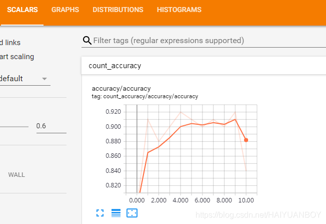

如果 loss 震动得比较厉害，可能是学习率设置太大

查看权值和偏置的 histogram 分布

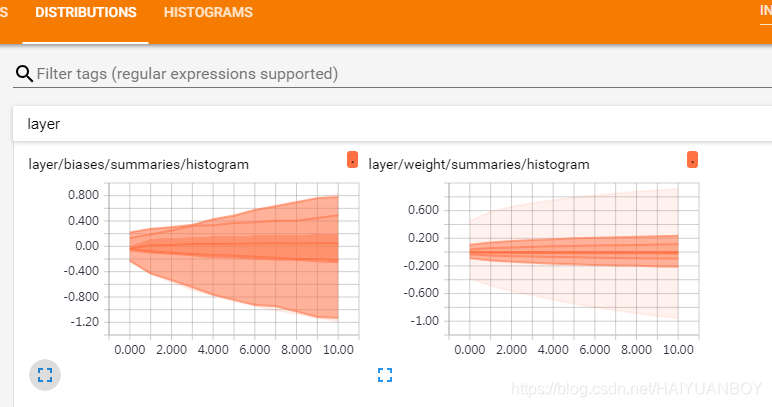
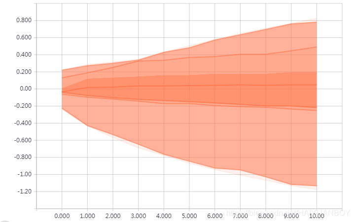
颜色越深表示在此范围分布越多

可视化

在项目下创建 projector 文件夹，projector 下创建 data 和 projector 文件夹，data 下放图片 mnist_10k_sprite.png

import tensorflow as tf
from tensorflow.examples.tutorials.mnist import input_data
# 载入数据集
mnist = input_data.read_data_sets('MNIST_data',one_hot=True)

# 运行次数
max_steps = 1001
# 图片数量
image_num = 3000
# 文件路径
DIR = 'D:/notebook/py3/'

# 定义会话
sess = tf.Session()

# 载入图片，stack方法把图片追加进来
embedding = tf.Variable(tf.stack(mnist.test.images[:image_num]), trainable=False, name='embedding')

# 参数概要
def variable_summaries(var):
    with tf.name_scope('summaries'):
        mean = tf.reduce_mean(var)
        # scalar 记录这个值，且起名字
        tf.summary.scalar('mean', mean)
        with tf.name_scope('summaries'):
            stddev = tf.sqrt(tf.reduce_mean(tf.square(var - mean))) # 标准差
        tf.summary.scalar('stddev', stddev)
        tf.summary.scalar('max', tf.reduce_max(var))
        tf.summary.scalar('min', tf.reduce_min(var))
        tf.summary.histogram('histogram', var) # 直方图

#命名空间
with tf.name_scope('input'):
    #这里的none表示第一个维度可以是任意的长度
    x = tf.placeholder(tf.float32,[None,784],name='x-input')
    #正确的标签
    y = tf.placeholder(tf.float32,[None,10],name='y-input')
    
#显示图片
with tf.name_scope('input_reshape'):
    # -1 代表不确定的，任意的值，把 784 转化为 28 * 28，维度是 1，因为是黑白图片，彩色维度 3
    image_shaped_input = tf.reshape(x, [-1, 28, 28, 1]) 
    # 放 10 张图片
    tf.summary.image('input', image_shaped_input, 10)
    
with tf.name_scope('layer'):
    #创建一个简单神经网络
    with tf.name_scope('weights'):
        W = tf.Variable(tf.zeros([784,10]),name='W')
        variable_summaries(W)
    with tf.name_scope('biases'):
        b = tf.Variable(tf.zeros([10]),name='b')
        variable_summaries(b)
    with tf.name_scope('wx_plus_b'):
        wx_plus_b = tf.matmul(x,W) + b
    with tf.name_scope('softmax'):    
        prediction = tf.nn.softmax(wx_plus_b)
        
with tf.name_scope('loss'):
    # 交叉熵代价函数配合 softmax 使用
    # 因为 prediction 是通过 softmax 来的，它是类别概率数组，所以不能直接用普通的交叉熵函数
    loss = tf.reduce_mean(tf.nn.softmax_cross_entropy_with_logits(labels=y,logits=prediction))
    tf.summary.scalar('loss',loss)
with tf.name_scope('train'):
    #使用梯度下降法
    train_step = tf.train.GradientDescentOptimizer(0.5).minimize(loss)
    
#初始化变量
sess.run(tf.global_variables_initializer())

with tf.name_scope('accuracy'):
    with tf.name_scope('correct_prediction'):
        #结果存放在一个布尔型列表中
        correct_prediction = tf.equal(tf.argmax(y,1),tf.argmax(prediction,1))#argmax返回一维张量中最大的值所在的位置
    with tf.name_scope('accuracy'):
        #求准确率
        accuracy = tf.reduce_mean(tf.cast(correct_prediction,tf.float32))#把correct_prediction变为float32类型
        tf.summary.scalar('accuracy',accuracy)
        
#产生metadata文件
if tf.gfile.Exists(DIR + 'projector/projector/metadata.tsv'):
    tf.gfile.DeleteRecursively(DIR + 'projector/projector/metadata.tsv')
with open(DIR + 'projector/projector/metadata.tsv', 'w') as f:
    labels = sess.run(tf.argmax(mnist.test.labels[:],1))
    for i in range(image_num):   
        f.write(str(labels[i]) + '\n')        
        
#合并所有的summary
merged = tf.summary.merge_all()

projector_writer = tf.summary.FileWriter(DIR + 'projector/projector',sess.graph)
# 保存网络的模型
saver = tf.train.Saver()
config = projector.ProjectorConfig()
embed = config.embeddings.add()
embed.tensor_name = embedding.name
embed.metadata_path = DIR + 'projector/projector/metadata.tsv'
embed.sprite.image_path = DIR + 'projector/data/mnist_10k_sprite.png'
embed.sprite.single_image_dim.extend([28,28])
projector.visualize_embeddings(projector_writer,config)

for i in range(max_steps):
    #每个批次100个样本
    batch_xs,batch_ys = mnist.train.next_batch(100)
    run_options = tf.RunOptions(trace_level=tf.RunOptions.FULL_TRACE)
    run_metadata = tf.RunMetadata()
    sess.run(train_step,feed_dict={x:batch_xs,y:batch_ys},options=run_options,run_metadata=run_metadata)
    summary = sess.run(merged,feed_dict={x:batch_xs,y:batch_ys},options=run_options,run_metadata=run_metadata)
    # 记录参数的变化
    projector_writer.add_run_metadata(run_metadata, 'step%03d' % i)
    projector_writer.add_summary(summary, i)
    
    if i%100 == 0:
        acc = sess.run(accuracy,feed_dict={x:mnist.test.images,y:mnist.test.labels})
        print ("Iter " + str(i) + ", Testing Accuracy= " + str(acc))

# 保存模型
saver.save(sess, DIR + 'projector/projector/a_model.ckpt', global_step=max_steps)
projector_writer.close()
sess.close()

运行

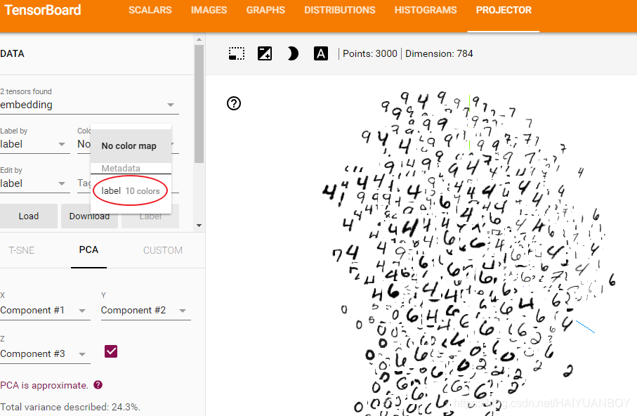
跑模型，查看迭代次数