


一、概念
The multiple comparison procedures all allow for examining aspects of superior predictive ability.
用于检验更优的预测能力
There are three available:
SPA- The test of Superior Predictive Ability, also known as the Reality Check (and accessible asRealityCheck) or the bootstrap data snooper, examines whether any model in a set of models can outperform a benchmark.- 检验一系列模型能够优于基本模型
StepM- The stepwise multiple testing procedure uses sequential testing to determine which models are superior to a benchmark.- 使用连续的检验决定哪个模型优于基准模型
MCS- The model confidence set which computes the set of models which with performance indistinguishable from others in the set.- 计算与模型集中性能相仿的模型
All procedures take losses as inputs. That is, smaller values are preferred to larger values. This is common when evaluating forecasting models where the loss function is usually defined as a positive function of the forecast error that is increasing in the absolute error. Leading examples are Mean Square Error (MSE) and Mean Absolute Deviation (MAD).
所有的方法都以Losses作为输入。即,越小越好。当评估预测模型性能时,Loss函数通常被定义为预测误差的正函数,随着绝对误差上升而上升。典型的例子为均方误差和均值绝对误差。
二、SPA Test
1、概念
This procedure requires a t-element array of benchmark losses and a t by k-element array of model losses. The null hypothesis is that no model is better than the benchmark, or
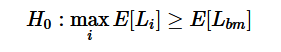
SPA算法的假设:没有模型优于基准模型。。
where Li is the loss from model i and Lbm is the loss from the benchmark model.
其中Li为模型i的Loss,公式左侧代表多个模型损失的均值;同理,Lbm代表基准模型损失。
This procedure is normally used when there are many competing forecasting models such as in the study of technical trading rules. The example below will make use of a set of models which are all equivalently good to a benchmark model and will serve as a size study.
该模型一般用于评估多个算法的优劣。
2、例子
Study Design
The study will make use of a measurement error in predictors to produce a large set of correlated variables that all have equal expected MSE.
本例将使用预设误差的预测因子,产生一系列相关变量,且其具有相同的MSE(LOSS)。
The benchmark will have identical measurement error and so all models have the same expected loss, although will have different forecasts.
基准模型和其他模型一样具有形同误差,尽管其预测值不同。
The first block computed the series to be forecast.
(1)首先生成被预测值,真实y。
import statsmodels.api as sm
from numpy.random import randn
t = 1000
#随机生产1000*3的因子,1000为时间序列长度
factors = randn(t, 3)
beta = np.array([1, 0.5, 0.1])
#e为残差
e = randn(t)
#y为被预测值
y = factors.dot(beta)
(2)再计算包含噪音的模型因子:1+500。该模型通过前500个时间序列拟合,再通过后500个时间序列预测,从而计算Loss。
The next block computes the benchmark factors and the model factors by contaminating the original factors with noise. The models are estimated on the first 500 observations and predictions are made for the second 500. Finally, losses are constructed from these predictions.
# 设置基准模型
# 生成基准模型因子=真实因子+噪音 1000*3维
bm_factors = factors + randn(t, 3)
# 通过前500个时间序列回归得beta
bm_beta = sm.OLS(y[:500], bm_factors[:500]).fit().params
# 通过后500个时间序列计算Loss
bm_losses = (y[500:] - bm_factors[500:].dot(bm_beta)) ** 2.0

# 设定500个比较模型
k = 500
model_factors = np.zeros((k, t, 3))
model_losses = np.zeros((500, k))
for i in range(k):
    # 给每个模型加噪音
    model_factors[i] = factors + randn(1000, 3)
    # 计算beta
    model_beta = sm.OLS(y[:500], model_factors[i, :500]).fit().params
    # 预测计算Loss,该矩阵维度为500*500,即时间序列*模型数量,每一列是一个模型的Loss
    model_losses[:, i] = (y[500:] - model_factors[i, 500:].dot(model_beta)) ** 2.0
(3)最终,我们可以使用SPA了。SPA要求基准模型以及竞争模型的Loss作为输入。其他的输入选项可以进行自助抽样法,或者是其他对于Loss的Student化。
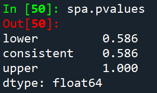
Finally the SPA can be used. The SPA requires the losses from the benchmark and the models as inputs. Other inputs allow the bootstrap sued to be changed or for various options regarding studentization of the losses. compute does the real work, and then pvalues contains the probability that the null is true given the realizations.
本例中,我们无法拒绝原假设。三个P值对应于不同Loss的re-centerings。我们通常使用consistent的P值。
In this case, one would not reject. The three p-values correspond to different re-centerings of the losses. In general, the consistent p-value should be used. It should always be the case that
![]()
from arch.bootstrap import SPA

spa = SPA(bm_losses, model_losses, seed=seed)
spa.compute()
spa.pvalues
3、进阶
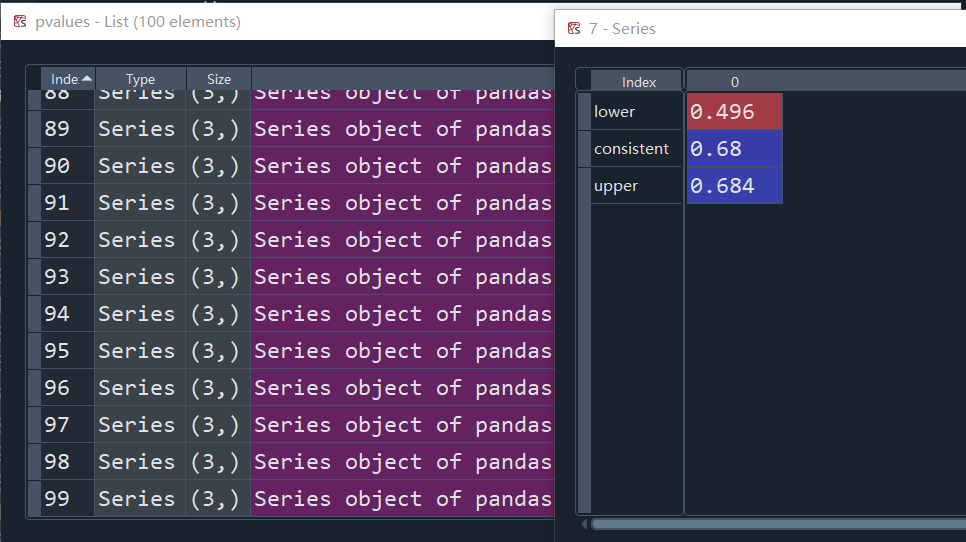
上述过程可以重复多次以进行模拟。这里因为时间关系,我们只重复100次。并且,在每一次SPA的应用中,我设定250为Bootstrap复制次数,默认值为1000。
The same blocks can be repeated to perform a simulation study. Here I only use 100 replications since this should complete in a reasonable amount of time. Also I set reps=250 to limit the number of bootstrap replications in each application of the SPA (the default is a more reasonable 1000).
# Save the pvalues
pvalues = []
# 设定重复次数
b = 100
seeds = gen.integers(0, 2 ** 31 - 1, b)
# Repeat 100 times
for j in range(b):
    if j % 10 == 0:
        print(j)
	#设定真实y
    factors = randn(t, 3)
    beta = np.array([1, 0.5, 0.1])
    e = randn(t)
    y = factors.dot(beta)

	#计算基准模型损失
    # Measurement noise
    bm_factors = factors + randn(t, 3)
    # Fit using first half, predict second half
    bm_beta = sm.OLS(y[:500], bm_factors[:500]).fit().params
    # MSE loss
    bm_losses = (y[500:] - bm_factors[500:].dot(bm_beta)) ** 2.0
    # Number of models

	#计算检验模型损失
    k = 500
    model_factors = np.zeros((k, t, 3))
    model_losses = np.zeros((500, k))
    for i in range(k):
        model_factors[i] = factors + randn(1000, 3)
        model_beta = sm.OLS(y[:500], model_factors[i, :500]).fit().params
        # MSE loss
        model_losses[:, i] = (y[500:] - model_factors[i, 500:].dot(model_beta)) ** 2.0

	#使用Bootstrap
	# Lower the bootstrap replications to 250
    spa = SPA(bm_losses, model_losses, reps=250, seed=seeds[j])
    spa.compute()
    pvalues.append(spa.pvalues)
最终,我们得到了100个SPA结果。
最终,我们画出P值。理想情况下,该曲线应为45度,表现size是正确的。
注意:在每次循环中,SPA的值是随着j而变化的,因此希望成45度。
spa = SPA(bm_losses, model_losses, reps=250, seed=seeds[j])
Finally the pvalues can be plotted. Ideally they should form a 45o line indicating the size is correct. Both the consistent and upper perform well. The lower has too many small p-values.
4、SPA可以拒绝零假设。
The SPA also has power to reject then the null is violated. The simulation will be modified so that the amount of measurement error differs across models, and so that some models are actually better than the benchmark. The p-values should be small indicating rejection of the null.
# Number of models
k = 500
model_factors = np.zeros((k, t, 3))
model_losses = np.zeros((500, k))
for i in range(k):
    # K越大的模型,噪声越小
    scale = (2500.0 - i) / 2500.0
    model_factors[i] = factors + scale * randn(1000, 3)
    model_beta = sm.OLS(y[:500], model_factors[i, :500]).fit().params
    # MSE loss
    model_losses[:, i] = (y[500:] - model_factors[i, 500:].dot(model_beta)) ** 2.0

spa = SPA(bm_losses, model_losses, seed=seed)
spa.compute()
spa.pvalues
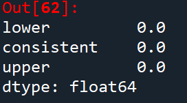
P值很小,可以拒绝零假设。
我们画出平均Loss,以验证说法。
Here the average losses are plotted. The higher index models are clearly better than the lower index models -- and the benchmark model (which is identical to model.0).
#计算出500个模型的Loss
model_losses = pd.DataFrame(model_losses, columns=["model." + str(i) for i in range(k)])
#取时间序列均值,得到各模型的Loss
avg_model_losses = pd.DataFrame(model_losses.mean(0), columns=["Average loss"])
fig = avg_model_losses.plot(style=["o"])
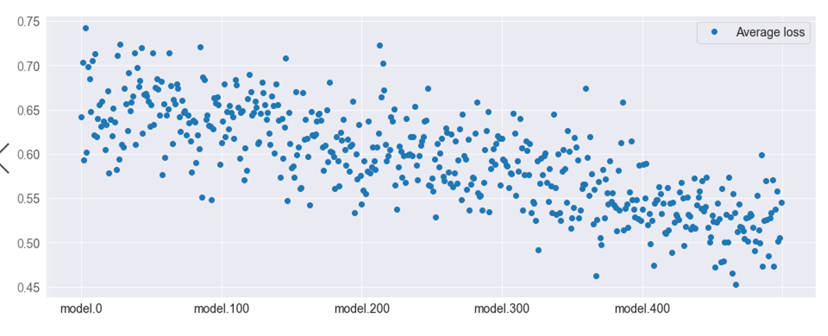
显然,K越大的模型Loss越小,且大多优于基准模型(与model一致,其噪声的系数都为1)。


 2万+
2万+


 到【灌水乐园】发言


