Task4:建模调参

Task4:建模调参

一，线性回归模型

线性回归是利用数理统计中回归分析，来确定两种或两种以上变量间相互依赖的定量关系的一种统计分析方法，运用十分广泛。其表达形式为y = w’x+e，e为误差服从均值为0的正态分布。（百度百科）
线性回归模型是目前最常用，运用最广泛的一个模型，在数学，计算机学，金融学，经济学，流行病学等多个领域都有广泛运用，而且我接触到的线性回归问题也较多，所以这次主要学习了线性回归模型。
线性回归主要涉及到损失函数、优化方法、梯度下降等问题

二，通过Python3分析

1，读取数据

import pandas as pd
import numpy as np
import warnings
warnings.filterwarnings('ignore')

def reduce_mem_usage(df):
    """ iterate through all the columns of a dataframe and modify the data type
        to reduce memory usage.        
    """
    start_mem = df.memory_usage().sum() 
    print('Memory usage of dataframe is {:.2f} MB'.format(start_mem))
    
    for col in df.columns:
        col_type = df[col].dtype
        
        if col_type != object:
            c_min = df[col].min()
            c_max = df[col].max()
            if str(col_type)[:3] == 'int':
                if c_min > np.iinfo(np.int8).min and c_max < np.iinfo(np.int8).max:
                    df[col] = df[col].astype(np.int8)
                elif c_min > np.iinfo(np.int16).min and c_max < np.iinfo(np.int16).max:
                    df[col] = df[col].astype(np.int16)
                elif c_min > np.iinfo(np.int32).min and c_max < np.iinfo(np.int32).max:
                    df[col] = df[col].astype(np.int32)
                elif c_min > np.iinfo(np.int64).min and c_max < np.iinfo(np.int64).max:
                    df[col] = df[col].astype(np.int64)  
            else:
                if c_min > np.finfo(np.float16).min and c_max < np.finfo(np.float16).max:
                    df[col] = df[col].astype(np.float16)
                elif c_min > np.finfo(np.float32).min and c_max < np.finfo(np.float32).max:
                    df[col] = df[col].astype(np.float32)
                else:
                    df[col] = df[col].astype(np.float64)
        else:
            df[col] = df[col].astype('category')

    end_mem = df.memory_usage().sum() 
    print('Memory usage after optimization is: {:.2f} MB'.format(end_mem))
    print('Decreased by {:.1f}%'.format(100 * (start_mem - end_mem) / start_mem))
    return df

sample_feature = reduce_mem_usage(pd.read_csv('data_for_tree.csv'))

Memory usage of dataframe is 60507328.00 MB

Memory usage after optimization is: 15724107.00 MB

Decreased by 74.0%

continuous_feature_names = [x for x in sample_feature.columns if x not in ['price','brand','model','brand']]

2，线性回归

（1）、简单建模

from sklearn.linear_model import LinearRegression

model = LinearRegression(normalize=True)

model = model.fit(train_X, train_y)

查看训练的线性回归模型的截距与权重
[(‘v_6’, 3342612.384537345),
, (‘v_8’, 684205.534533214),
, (‘v_9’, 178967.94192530424),
, (‘v_7’, 35223.07319016895),
, (‘v_5’, 21917.550249749802),
, (‘v_3’, 12782.03250792227),
, (‘v_12’, 11654.925634146672),
, (‘v_13’, 9884.194615297649),
, (‘v_11’, 5519.182176035517),
, (‘v_10’, 3765.6101415594258),
, (‘gearbox’, 900.3205339198406),
, (‘fuelType’, 353.5206495542567),
, (‘bodyType’, 186.51797317460046),
, (‘city’, 45.17354204168846),
, (‘power’, 31.163045441455335),
, (‘brand_price_median’, 0.535967111869784),
, (‘brand_price_std’, 0.4346788365040235),
, (‘brand_amount’, 0.15308295553300566),
, (‘brand_price_max’, 0.003891831020467389),
, (‘seller’, -1.2684613466262817e-06),
, (‘offerType’, -4.759058356285095e-06),
, (‘brand_price_sum’, -2.2430642281682917e-05),
, (‘name’, -0.00042591632723759166),
, (‘used_time’, -0.012574429533889028),
, (‘brand_price_average’, -0.414105722833381),
, (‘brand_price_min’, -2.3163823428971835),
, (‘train’, -5.392535065078232),
, (‘power_bin’, -59.24591853031839),
, (‘v_14’, -233.1604256172217),
, (‘kilometer’, -372.96600915402496),
, (‘notRepairedDamage’, -449.29703564695365),
, (‘v_0’, -1490.6790578168238),
, (‘v_4’, -14219.648899108111),
, (‘v_2’, -16528.55239086934),
, (‘v_1’, -42869.43976200439)]

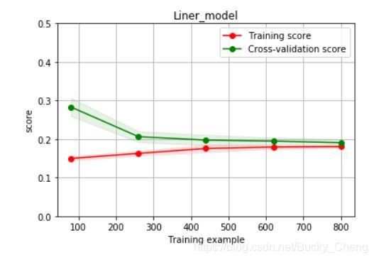
（2）、绘制曲线

from sklearn.model_selection import learning_curve, validation_curve

? learning_curve

def plot_learning_curve(estimator, title, X, y, ylim=None, cv=None,n_jobs=1, train_size=np.linspace(.1, 1.0, 5 )):  
    plt.figure()  
    plt.title(title)  
    if ylim is not None:  
        plt.ylim(*ylim)  
    plt.xlabel('Training example')  
    plt.ylabel('score')  
    train_sizes, train_scores, test_scores = learning_curve(estimator, X, y, cv=cv, n_jobs=n_jobs, train_sizes=train_size, scoring = make_scorer(mean_absolute_error))  
    train_scores_mean = np.mean(train_scores, axis=1)  
    train_scores_std = np.std(train_scores, axis=1)  
    test_scores_mean = np.mean(test_scores, axis=1)  
    test_scores_std = np.std(test_scores, axis=1)  
    plt.grid()#区域  
    plt.fill_between(train_sizes, train_scores_mean - train_scores_std,  
                     train_scores_mean + train_scores_std, alpha=0.1,  
                     color="r")  
    plt.fill_between(train_sizes, test_scores_mean - test_scores_std,  
                     test_scores_mean + test_scores_std, alpha=0.1,  
                     color="g")  
    plt.plot(train_sizes, train_scores_mean, 'o-', color='r',  
             label="Training score")  
    plt.plot(train_sizes, test_scores_mean,'o-',color="g",  
             label="Cross-validation score")  
    plt.legend(loc="best")  
    return plt 

plot_learning_curve(LinearRegression(), 'Liner_model', train_X[:1000], train_y_ln[:1000], ylim=(0.0, 0.5), cv=5, n_jobs=1) 

3，模型调参

建模调参主要有
贪心调参 https://www.jianshu.com/p/ab89df9759c8.
Grid Search调参https://blog.youkuaiyun.com/weixin_43172660/article/details/83032029.
贝叶斯调参https://blog.youkuaiyun.com/linxid/article/details/81189154.
具体的代码案例分析可见: https://tianchi.aliyun.com/notebook-ai/detail?spm=5176.12586969.1002.18.1cd8593aw4bbL5&postId=95460.