曹健老师 TensorFlow2.1 —— 第六章循环神经网络_from tensorflow.keras.layers import dropout, dense-优快云博客

本文链接：https://blog.youkuaiyun.com/Amber__py/article/details/116009881

本文详细介绍了如何使用RNN、LSTM和GRU在股票价格预测中进行连续数据建模，包括模型构建、参数调整、训练过程和实际预测示例。从数据预处理到模型构建，展示了从独热编码到Embedding编码的转换，以及不同类型的循环神经网络在时间序列预测中的优势和区别。

摘要生成于 C知道，由 DeepSeek-R1 满血版支持，前往体验 >

本章目的：用 RNN 实现连续数据的预测 ( 以股票预测为例 ).

6.1 循环核

循环核：具有记忆力，通过不同时刻的参数共享，实现了对时间序列的信息提取。循环核如下图所示，圆柱为记忆体，记忆体下面、侧面、上面分别有三组待训练的参数矩阵. 记忆体个数可被指定，改变记忆体容量，当记忆体个数被指定，输入 $x_{t}$ 、输出 $y_{t}$ 维度被指定，周围待训练参数的维度也就被限定了. 记忆体内存储着每个时刻的状态信息为 $h_{t}$ ，当前时刻循环核的输出特征为 $y_{t}$ ，计算公式为：

$h_{t} = tanh(x_{t}w_{xh}+h_{t-1}w_{hh}+bh)$

$y_{t} = softmax(h_{t}w_{hy}+by)$

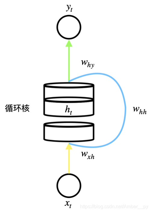
在前向传播时，记忆体内存储的状态信息 $h_{t}$ 在每个时刻都被刷新，三个参数矩阵 $w_{xh}$ 、 $w_{hh}$ 、 $w_{hy}$ 自始至终都是固定不变的，只有当反向传播时，三个参数矩阵才会被梯度下降法更新.

6.2 循环核时间步展开

按照时间步展开，就是把循环核按照时间轴方向展开，可以表示为下图：

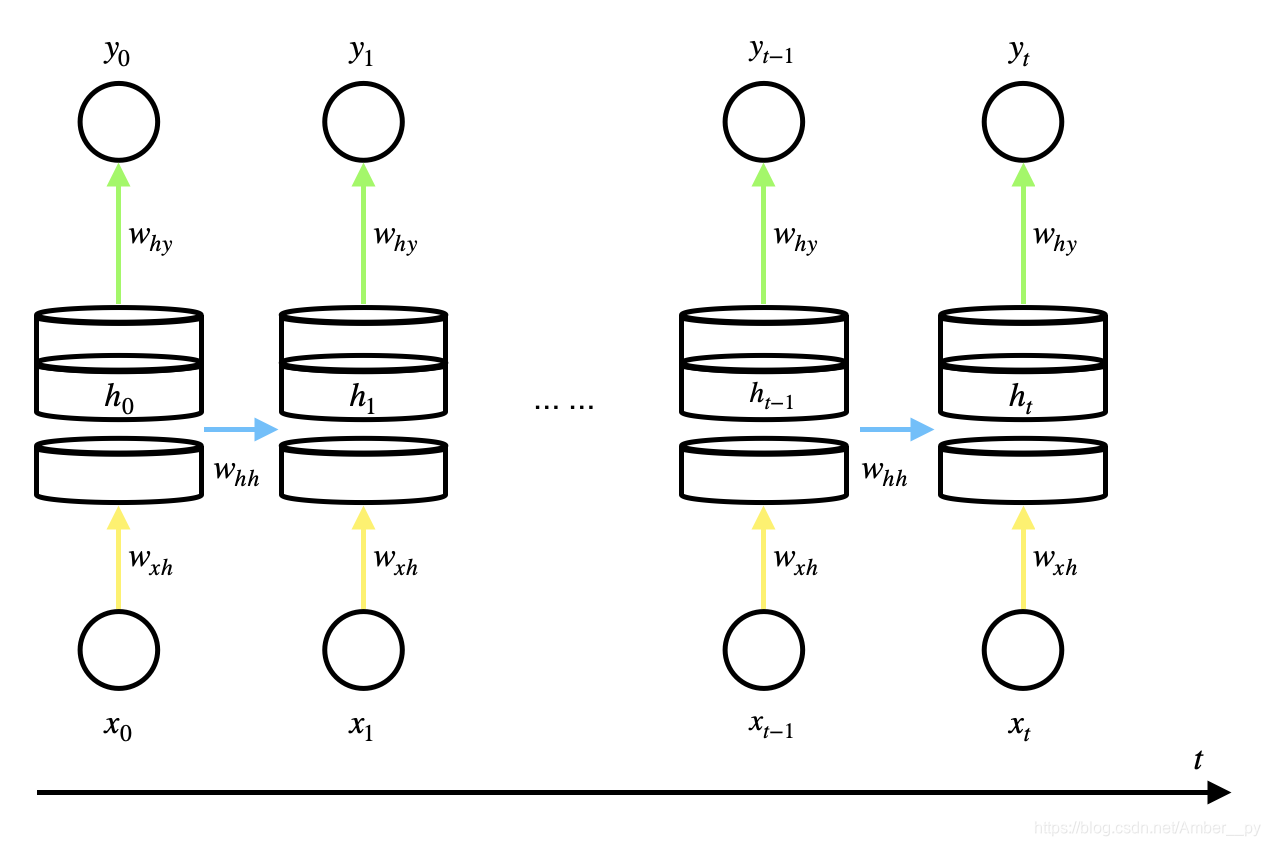
每个时刻记忆体状态信息被刷新，参数矩阵固定不变，训练的目的是优化这三个参数矩阵，以找到效果最好的参数矩阵，用其执行前向传播，输出预测结果.

循环神经网络即借助循环核实现时间特征的提取，送入全连接网络，实现连续数据的预测.

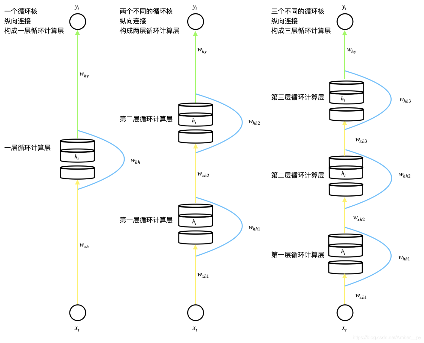
6.3 循环计算层

每个循环核构成一层循环计算层，循环计算层的层数是向输出方向增长的. 如下图所示，其中，每个循环核中记忆体的个数根据需求任意指定.

6.4 TF 描述循环计算层的

tf.keras.layers.SimpleRNN(记忆体个数, activation='激活函数', return_sequences=是否每个时刻输出 ht 到下一层)
activation 默认为 tanh      # 计算 ht
return_sequences = True    # 各时间输出 ht
return_sequences = False   # 仅最后时间步输出 ht ( 默认 )
# 一般中间层的循环核用 True, 每个时间步都把 ht 输出给下一层, 最后一层的循环核用 False
例如：
SimpleRNN(3, return_sequences=True)

API 对送入循环层的数据维度是有要求的，要求送入循环层的维度是三维的：

x_train 维度: [送入样本数, 循环核时间展开步数, 每个时间步输入特征个数]

6.5 循环计算过程 I

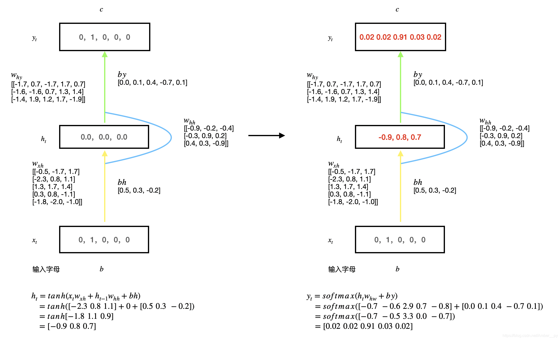
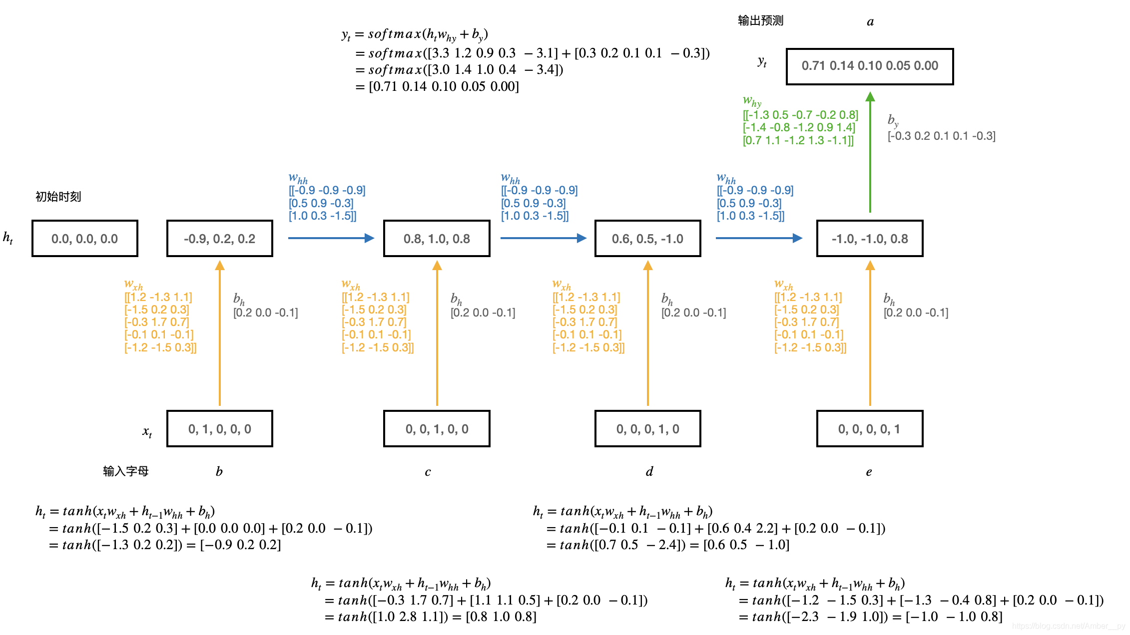
以字母预测为例：( 输入 a 预测出 b，输入 b 预测出 c，输入 c 预测出 d，输入 d 预测出 e，输入 e 预测出 a )

神经网络的输入都是数字，首先要把用到的字母 a 、b 、c 、d 、e 用独热编码进行编码，如下表所示：

词向量空间
10000	a
01000	b
00100	c
00010	d
00001	e

然后随机生成 $w_{xh}$ 、 $w_{hh}$ 、 $w_{hy}$ 三个参数矩阵，记忆体个数选取 3 ，具体计算过程如下图：

代码实现，按照六步法

首先 import 相关模块

import numpy as np
import tensorflow as tf
from tensorflow.keras.layers import Dense, SimpleRNN
import matplotlib.pyplot as plt
import os

数据

input_word = "abcde"
w_to_id = {'a':0, 'b':1, 'c':2, 'd':3, 'e':4}    # 单词映射到数值 id 的词典
id_to_onehot = {0:[1., 0., 0., 0., 0.], 1:[0., 1., 0., 0., 0.], 2:[0., 0., 1., 0., 0.], 3:[0., 0., 0., 1., 0.],4:[0., 0., 0., 0., 1.]}    # id 编码为 one-hot

x_train = [id_to_onehot[w_to_id['a']], id_to_onehot[w_to_id['b']], id_to_onehot[w_to_id['c']], id_to_onehot[w_to_id['d']], id_to_onehot[w_to_id['e']]]
y_train = [w_to_id['b'], w_to_id['c'], w_to_id['d'], w_to_id['e'], w_to_id['a']]

np.random.seed(7)
np.random.shuffle(x_train)
np.random.seed(7)
np.random.shuffle(y_train)
tf.random.set_seed(7)

# 使 x_train 符合 SimpleRNN 输入要求：[送入样本数, 循环核时间展开步数, 每个时间步输入特征个数]
# 此处整个数据集送入，因此送入样本数为 len(x_train); 输入 1 个字母出结果，所以循环核展开步数为 1 ;表示为独热编码有 5 个输入特征，所以每个时间步输入特征个数为 5
x_train = np.reshape(x_train, (len(x_train)), 1, 5)
y_trian = np.array(y_train)

Sequential

# 搭建具有三个记忆体的循环层 记忆体个数可自行调整，记忆体个数越多，记忆力越好，但占用资源会更多
# 记忆体个数 = 隐藏层神经元个数 = 隐状态的维度
model = tf.keras.Sequential([
    SimpleRNN(3),
    Dense(5, activation='softmax')
])

Compile

model.complie(optimizer=tf.keras.optimizers.Adam(0.01),
              loss=tf.keras.losses.SparseCategoricalCrossentropy(from_logits=False),
              metrics=['sparse_categorical_accuracy'])

checkpoint_save_path = "./checkpoint/rnn_onehot_1pre1.ckpt"

if os.path.exsits(checkpoint_save_path + ".index"):
    print("--------load the model--------")

cp_callback = tf.keras.callbacks.ModelCheckpoint(filepath=checkpoint_save_path,
                                                 save_weights_only=True,
                                                 save_best_only=True,
                                                 monitor='loss')    # 由于 fit 没有给出测试集，不计算测试集准确率，根据 loss ，保存最优模型

Fit

history = model.fit(x_train, y_train, batch_size=32, epochs=100, callbacks=[cp_callback])

Summary

model.summary()

应用：字母预测

# 先输入要执行几次预测任务
preNum = int(input("input the number of test alphabet:"))
for i in range(preNum):
    alphabet1 = input("input test alphabet:")
    alphabet = [id_to_onehot[w_to_id[aplhabet1]]]
    # 使 alphabet 符合 SimpleRNN 输入要求
    # 慈湖验证效果送入一个样本，所以送入样本数为 1; 输入一个字母出结果，所以循环核时间展开步数为 1; 表示为独热编码有 5 个输入特征，所以每个时间步输入特征个数为 5
    alphabet = np.reshape(alphabet, (1, 1, 5))
    result = model.predict(alphabet)
    pred = tf.argmax(result, axis=1)
    pred = int(pred)
    tf.print(alphabet1 + "->" + input_word[pred])

6.6 循环计算过程 II

把时间核按时间步展开，连续输入多个字母预测下一个字母. 以连续输入四个字母，预测下一个字母为例. 使用三个记忆体，用一套训练好的参数矩阵，计算过程参数矩阵不变，记忆体时刻更新，计算过程如下图：

代码实现

生成训练用的输入特征和标签

x_train = [
    [id_to_onehot[w_to_id['a']], id_to_onehot[w_to_id['b']], id_to_onehot[w_to_id['c']], id_to_onehot[w_to_id['d']]],
    [id_to_onehot[w_to_id['b']], id_to_onehot[w_to_id['c']], id_to_onehot[w_to_id['d']], id_to_onehot[w_to_id['e']]],
    [id_to_onehot[w_to_id['c']], id_to_onehot[w_to_id['d']], id_to_onehot[w_to_id['e']], id_to_onehot[w_to_id['a']]],
    [id_to_onehot[w_to_id['d']], id_to_onehot[w_to_id['e']], id_to_onehot[w_to_id['a']], id_to_onehot[w_to_id['b']]],
    [id_to_onehot[w_to_id['e']], id_to_onehot[w_to_id['a']], id_to_onehot[w_to_id['b']], id_to_onehot[w_to_id['c']]],
]
y_train = [w_to_id['e'], w_to_id['a'], w_to_id['b'], w_to_id['c'], w_to_id['d']]

# 把输入特征变为 RNN 层期待的形状, 其中，4 为循环核展开步数
# 因为 4 个字母通过 4 个连续的时刻送入网络，所以时间展开步数是 4 
x_train = np.reshape(x_train, (len(x_train), 4, 5))
y_train = np.array(y_train)

六步法，与循环计算过程 I 相同
应用：字母预测

preNum = int(input("input the number of test alphabet:"))
for i in range(preNum):
    alphabet1 = input("input the test alphaber:")
    alphabet = [id_to_onehot[w_to_id[a]] for a in alphabet1]
    # 使用 alphabet 符合 SimpleRNN 期待形状 
    alphabet = np.reshape(alphabet, (1, 4, 5))
    result = model.predict([alphabet])
    pred = tf.argmax(result, axis=1)
    pred = int(pred)
    tf.print(alphabet1 + "->" + input_word[pred])

6.7 Embedding 编码

独热编码：位宽与词汇量一致. 数据量大，过于稀疏，映射之间是独立的，没有表现出关联性.
Embedding：是一种单词编码方法，用低维向量实现了编码，通过神经网络训练优化，能够表达出单词间的相关性.

tf.keras.layers.Embedding(词汇表大小, 编码难度)
# 编码难度就是用几个数字表达一个单词

# 例如
tf.keras.layers.Embedding(100, 3)
# 对 1-100 进行编码，词汇表大小为 100 ，每个自然数用三个数字表示，编码维度为 3，[4] 的编码为 [0.25, 0.1, 0.11]
# 入 Embedding 时，x_train 维度：[送入样本数, 循环核时间展开步数]

用 Embedding 编码替换独热编码实现字母预测 ( 输入一个字母预测下一个字母 ) 任务

# 生成训练集输入特征和标签
x_train = [w_to_id['a'], w_to_id['b'], w_to_id['c'], w_to_id['d'], w_to_id['e']]
y_train = [w_to_id['b'], w_to_id['c'], w_to_id['d'], w_to_id['e'], w_to_id['a']]

# 把输入特征变为 Embedding 层期待的形状：[送入样本数, 循环核时间展开步数]
x_train = np.reshape(x_train, (len(x_train), 1))
y_train = np.array(y_train)

# Sequential 搭建网络结构时，增加 Embedding 层
model = tf.keras.Sequential([
    Embedding(5, 2),    # 对输入数据编码，这一层会生成一个五行两列的可训练参数矩阵 
    SimpleRNN(3),
    Dense(5, activation='softmax')
])

### 六步法 省略 ###

# 应用
preNum = int(input("input the number of test alphabet:"))
for i in range(preNum):
    alphabet1 = input("input test alphabet:")
    alphabet = [w_to_id[alphabet1]]
    alphabet = np.reshape(alphabet, (1, 1))
    result = model.predict(alphabet)
    pred = tf.argmax(result, axis=1)
    pred = int(pred)
    tf.print(alphabet1 + '->' + input_word[pred])

用 Embedding 编码替换独热编码实现字母预测 ( 输入四个字母预测下一个字母 ) 任务

# 把词汇量扩展到了 26 个
input_word = "abcdefghijklmnopqrstuvwxyz"
w_to_id = {'a':0, 'b':1, 'c':2, 'd':3, 'e':4, 'f':5, 'g':6, 'h':7,
            'i':8, 'j':9, 'k':10, 'l':11, 'm':12, 'n':13, 'o':14, 'p':15,'q':16, 
            'r':17, 's':18, 't':19, 'u':20, 'v':21, 'w':22, 'x':23, 'y':24, 'z':25}
training_set_scaled = [0, 1, 2, 3, 4, 5, 6, 7, 8, 9, 10,
                        11, 12, 13, 14, 15, 16, 17, 18, 19,
                          20, 21, 22, 23, 24, 25]
x_train = []
y_train = []

for i in rangw(4, 26):
    x_train.append(training_set_scaled[i-4:i])
    y_train.append(training_set_scaled[i])

# 把输入特征变成 Embedding 层期待的形状
x_train = np.reshape(x_train, (len(x_train), 4))
y_train = np.array(y_train)

# Sequential
model = tf.keras.Sequential([
    Embedding(26, 2),
    SimpleRNN(10),
    Dense(26, activation='softmax')
])

#### 六步法省略 ###

# 应用
preNum = int(input("input the number of test alphabet:"))
for i in range(preNum):
    alphabet1 = input("input test alphabet:")
    alphabet = [w_to_id[a] for a in alphabet1]
    alphabet = np.reshape(alphabet, (1, 4))
    result = model.predict([alphabet])
    pred = tf.argmax(result, axis=1)
    pred = int(pred)
    tf.print(alphabet1 + "->" + input_word[pred])

6.8 RNN 实现股票预测

使用 tushare 模块下载 SH600519 贵州茅台日 k 线数据，用连续 60 天的开盘价，预测第 61 天的开盘价.

import tushare as ts
df1 = ts.get_k_data('600519', ktype='D', start='2010-04-26', end='2020-04-26')
datapath1 = "./SH600519.csv"
df1.to_csv(datapath1)

六步法 —— import 相关模块

import numpy as np
import tensorflow as tf
from tensorflow.keras.layers import Dropout, Dense, SimpleRNN
import matplotlib.pyplot as plt
import os
import pandas as pd
from sklearn.preprocessing import MinMaxScaler
from sklearn.metrics import mean_squared_error, mean_absolute_error
import math

生成训练集和测试集

maotai = pd.read_csv("./SH600519.csv")
training_set = maotai.iloc[0:2426 - 300, 2:3].values
# 前 [2426-300=2126] 天的开盘价作为训练集，表格从 0 开始计数，2:3 是提取 [2:3) 列. 前闭后开，故提取出 c 列开盘价
test_set = maotai.iloc[2426-300:, 2:3].values   # 后 300 天的开盘价作为测试集
# 归一化, 使送入神经网络对数据分布在 0 到 1 之间
sc = MinMaxScaler(feature_range=(0, 1))     # 定义归一化：归一化到（0，1）之间
training_set_scaled = sc.fit_transform(training_set)    # 求得训练集的最大值、最小值，这些训练集固有的属性，并在训练集上进行归一化
test_set = sc.transform(test_set)   # 利用训练集的属性对测试集进行归一化
x_train = []
y_train = []
x_test = []
y_test = []

# 训练集：csv 表格中前 2426-300 = 2126 天数据
# 利用 for 循环，遍历整个训练集，提取训练集中连续 60 天的开盘价作为输入特征 x_train，第 61 天的数据作为标签 y_train，for 循环共构建 2426-300-60=2066 组数据.
for i in range(60, len(training_set_scaled)):
    x_train.append(training_set_scaled[i-60:i, 0])
    y_train.append(training_set_scaled[i, 0])
# 打乱训练集顺序
np.random.seed(7)
np.random.shuffle(x_train)
np.random.seed(7)
np.random.shuffle(y_train)
tf.random.set_seed(7)
# 将训练集由 list 格式转变为 array 格式
x_train, y_train = np.array(x_train), np.array(y_train)

# 使 x_train 符合 RNN 输入要求：[送入样本数, 循环核时间展开步数, 每个时间步输入特征个数].
# 此处整个数据集送入，送入样本数为 x_train.shape[0]即2066组数据，输入 60 个开盘价，循环核时间展开步数为 60 ；每个时间步送入的特征是某一天的开盘价，只有一个数据，故每个时间步输入特征个数为 1 .
x_train = np.reshape(x_train, (x_train.shape[0], 60, 1))
# 测试集：csv 表格中后 300 天数据
# 利用 for 循环，遍历整个测试集，提取测试集中连续 60 天的开盘价作为输入特征 x_train ，第 61 天的数据作为标签，for 循环共构建 300-60=240 组数据
for i in range(60, len(test_set)):
    x_test.append(test_set[i-60:i, 0])
    y_test.append(test_set[i, 0])
# 测试集变 array 并 reshape 为符合 RNN 输入要求
x_test, y_test = np.array(x_test), np.array(y_test)
x_test = np.reshape(x_test, (x_test.shape[0], 60, 1))

Sequential 搭建神经网络

model = tf.keras.Sequential([
    SimpleRNN(80, return_sequences=True),
    Dropout(0.2),
    SimpleRNN(100),
    Dropout(0.2),
    Dense(1)
])

Compile 配置训练方法

model.compile(optimizer=tf.keras.optimizers.Adam(0.001),
              loss='mean_squared_error')     # 损失函数使用均方误差
# 该应用只观测 loss 数值，不观测准确率，所以删去 metrics 选项，一会在每个 epoch 迭代显示时只显示 loss 值

设置断点续训

checkpoint_save_path = "./checkpoint/stock.ckpt"

if os.path.exists(checkpoint_save_path + ".index"):
    print("--------load the model--------")
    model.load_weights(checkpoint_save_path)

cp_callback = tf.keras.callbacks.ModelCheckpoint(filepath=checkpoint_save_path,
                                                 save_weights_only=True,
                                                 save_best_only=True,
                                                 monitor='val_loss')
history = model.fit(x_train, y_train, batch_size=64, epochs=50, validation_data=(x_test, y_test), validation_freq=1,
                        callbacks=[cp_callback])

summary 打印出网络结构和参数统计

model.summary()

参数提取和 loss 可视化

file = open('./weights.txt', 'w')
for v in model.trainable_variables:
    file.write(str(v.name) + '\n')
    file.write(str(v.shape) + '\n')
    file.write(str(v.numpy()) + '\n')
file.close()

loss = history.history['loss']
val_loss = history.history['val_loss']

plt.plot(loss, label='Training Loss')
plt.plot(val_loss, label='Validation Loss')
plt.title('Training and validation loss')
plt.legend()
plt.show()

用 predict 预测测试集数据

# 测试集输入模型进行预测
predict_stock_price = model.predict(x_test)
# 对预测数据还原 —— 从 (0, 1) 反归一化到原始范围
predict_stock_price = sc.inverse_transform(predict_stock_price)
# 对真实数据还原 —— 从 (0, 1) 反归一化到原始范围
real_stock_price = sc.inverse_transform(test_set[60:])
# 画出真实数据和预测数据的对比曲线
plt.plot(real_stock_price, color='red', label='MaoTai Stock Price')
plt.plot(predict_stock_price, color='blue', label='Predicted MaoTai Stock Price')
plt.title('MaoTai Stock Price Prediction')
plt.xlabel('Time')
plt.ylabel('MaoTai Stock Price')
plt.legend()
plt.show()

模型评价

# calculate MSE 均方误差 ——> E [(预测值-真实值)^2] 
mse = mean_squared_error(predict_stock_price, real_stock_price)
# calculate RMSE 均方根误差 ——> sqrt[MSE]
rmse = math.sqrt(mean_squared_error(predict_stock_price, real_stock_price))
# calculate MAE 平均绝对误差 ——> E[|预测值-真实值|]
mae = mean_absolute_error(predict_stock_price, real_stock_price)
print('均方误差：%.6f' % mse)
print('均方根误差：%.6f' % rmse)
print('平均绝对误差：%.6f' % mae)

6.9 LSTM 实现股票预测 ( LSTM 计算过程 _ TF 描述 LSTM 层 )

传统循环网络 RNN 可以通过记忆体实现短期记忆进行连续数据的预测，但当连续数据的序列变长时，会使展开时间步过长，在反向传播更新参数时，梯度按照时间步连续相乘，会导致梯度消失. LSTM ( 长短记忆网络 ) 由 Hochreither & Schmidhuber 于 1997 年提出，通过门控单元改善了 RNN 长期依赖问题. LSTM 引入了三个门限：

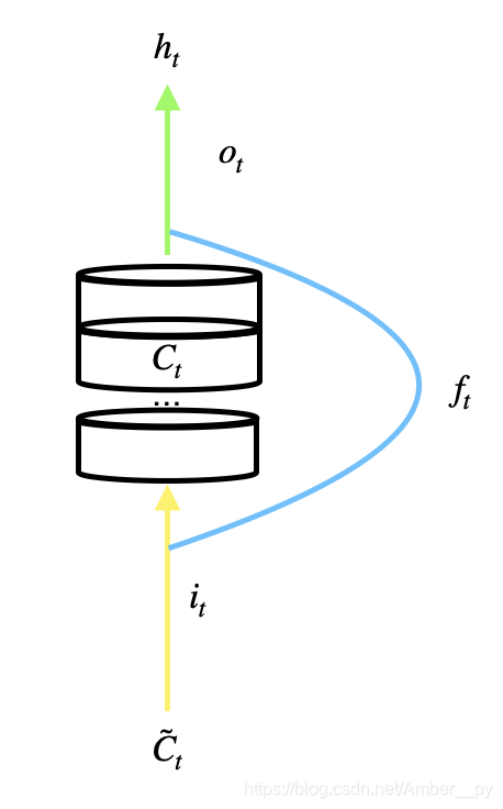
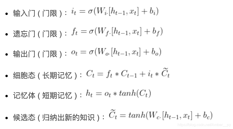
其中， $x_{t}$ 为当前时刻的输入特征， $h_{t-1}$ 为上一时刻的短期记忆， $W_{i},W_{f},W_{o}$ 是待训练参数矩阵， $b_{i},b_{f},b_{o}$ 是待训练偏置项， $\sigma$ 为 sigmoid 激活函数.

当有多层循环网络时，第二层的输入 $x_{t}$ 就是上一层循环网络的输出 $h_{t}$ ，输入第二层网络是第一层网络提取出的精华.

TF 描述 LSTM 层

tf.keras.layers.LSTM(记忆体个数, return_sequences=是否返回输出)
return_sequences=True 各时间步输出 ht
return_sequences=False 仅最后时间步输出 ht ( 默认 )
# 例如
model = tf.keras.Sequential([
    LSTM(80, return_sequences=True),
    Dropout(0.2),
    LSTM(100),
    Dropout(0.2),
    Dense(1)
])

LSTM 实现股票预测

# 导入 LSTM
from tensorflow.keras.layers import Dropout, Dense, LSTM

# 用 LSTM 层替换 RNN 层
model = tf.keras.Sequential([
    LSTM(80, return_sequences=True),
    Dropout(0.2),
    LSTM(100),
    Dropout(0.2),
    Dense(1)
])

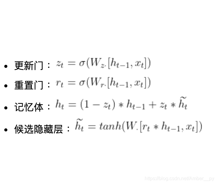
6.10 GRU 实现股票预测 ( GRU 计算过程 _ TF 描述 GRU 层 )

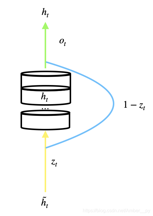
2014 年，Cho 等人简化了 LSTM 结构，提出了 GRU 网络，GRU 使记忆体 $h_{t}$ 融合了长期记忆和短期记忆， $h_{t}$ 包含了过去信息 $h_{t-1}$ 和现在的信息 $\widetilde{h_{t}}$ ，现在的信息 $\widetilde{h_{t}}$ 是过去信息 $h_{t-1}$ 过重置门与当前输入共同决定. 如下图所示. 前向传播时，直接使用记忆体更新公式，就可以算出每个时刻的 $h_{t}$ 值

TF 描述 GRU 层

tf.keras.layers.GRU(记忆体个数, return_sequences=是否返回输出)

GRU 实现股票预测

# import GRU 模块
from tensorflow.keras.layers import Dropout, Dense, GRU

# GRU 层替换 RNN 层
model = tf.keras.Sequential([
    GRU(80, return_sequences=True),
    Dropout(0.2),
    GRU(100),
    Dropout(0.2),
    Dense(1)
])