【再学Tensorflow2】TensorFlow2的张量操作与AutoGraph计算图

本文链接：https://blog.youkuaiyun.com/ARPOSPF/article/details/128468896

本文详细介绍了TensorFlow2中的张量操作，包括张量创建、索引切片、维度变换、数学运算等内容，并深入探讨了Autograph的工作原理及其与tf.Module的应用。

摘要生成于 C知道，由 DeepSeek-R1 满血版支持，前往体验 >

TensorFlow的低阶API主要包括张量操作，计算图和自动微分。在低阶API层次上，可以把TensorFlow当做一个增强版的numpy来使用。但TensorFlow提供的方法比numpy更全面，运算速度更快，如果需要的话，还可以使用 GPU进行加速。

TensorFlow2的张量操作主要包括张量的结构操作和张量的数学运算：

张量结构操作如：张量创建，索引切片，维度变换，合并分割。
张量数学运算主要有：标量运算，向量运算，矩阵运算。以及张量运算的广播机制。

对于Autograph计算图，将介绍使用Autograph的规范建议，Autograph的机制原理，Autograph和tf.Module。

Tensorflow中的张量操作

创建张量

基础操作：

import numpy as np
import tensorflow as tf
#%%
a = tf.constant([1,2,3],dtype=tf.float32)
tf.print(a)
#%%
b = tf.range(1,10, delta=2)
tf.print(b)
#%%
c = tf.linspace(0.0,2*3.14,100)
tf.print(c)
#%%
d = tf.zeros([3,3])
tf.print(d)
#%%
e = tf.ones([3,3])
f = tf.zeros_like(e, dtype=tf.float32)
tf.print(e)
tf.print(f)
#%%
g = tf.fill([3,2],5)
tf.print(g)

进阶操作：

# 均匀分布随机
tf.random.set_seed(1.0)
a = tf.random.uniform([5], minval=0, maxval=10)
tf.print(a)
#%%
# 正态分布随机
b = tf.random.normal([3,3],mean=0.0, stddev=1.0)
tf.print(b)
#%%
# 正态分布随机，删除2倍方差以外数据重新生成
c = tf.random.truncated_normal((5,5),mean=0.0,stddev=1.0,dtype=tf.float32)
tf.print(c)
#%%
# 特殊矩阵
I = tf.eye(3,3) # 单位矩阵
tf.print(I)
tf.print(' ')
t = tf.linalg.diag([1,2,3]) # 对角矩阵
tf.print(t)

索引与切片

张量的索引切片方式和numpy几乎是一样的。切片时支持缺省参数和省略号。

对于tf.Variable，可以通过索引和切片对部分元素进行修改。
对于提取张量的连续子区域，也可以使用tf.slice。
此外，对于不规则的切片提取，可以使用tf.gather，tf.gather_nd，tf.boolean_mask。
tf.boolean_mask功能最为强大，它可以实现tf.gather，tf.gather_nd的功能，并且tf.boolean_mask还可以实现布尔索引。
如果要通过修改张量的某些元素得到新的张量，可以使用tf.where，tf.scatter_nd。

tf.random.set_seed(1234)
t = tf.random.uniform([5,5],minval=0,maxval=10,dtype=tf.int32)
tf.print(t)
#%%
# 第0行
tf.print(t[0])
#%%
# 倒数第一行
tf.print(t[-1])
#%%
# 第1行第3列
tf.print(t[1,3])
tf.print(t[1][3])
#%%
# 第1行至第3行
tf.print(t[1:4,:])
tf.print(tf.slice(t, [1, 0], [3, 5])) # tf.slice(input, begin_vector, size_vector)
#%%
# 第1行至最后一行，第0列到最后一列每隔两列取一列
tf.print(t[1:4, :4:2])
#%%
# 对变量来说，可以使用索引和切片修改部分元素
x = tf.Variable([[1,2],[3,4]], dtype=tf.float32)
x[1,:].assign(tf.constant([0.0,0.0]))
tf.print(x)
#%%
a = tf.random.uniform([3,3,3],minval=0,maxval=10,dtype=tf.int32)
tf.print(a)
#%%
# 省略号可以表示多个冒号
tf.print(a[...,1])

以上切片方式相对规则，对于不规则的切片提取，可以使用tf.gather，tf.gather_nd，tf.boolean_mask。
示例：考虑班级成绩册的例子，有4个班级，每个班级10个学生，每个学生7门科目成绩。可以用一个4×10×7的张量来表示。
一个张量
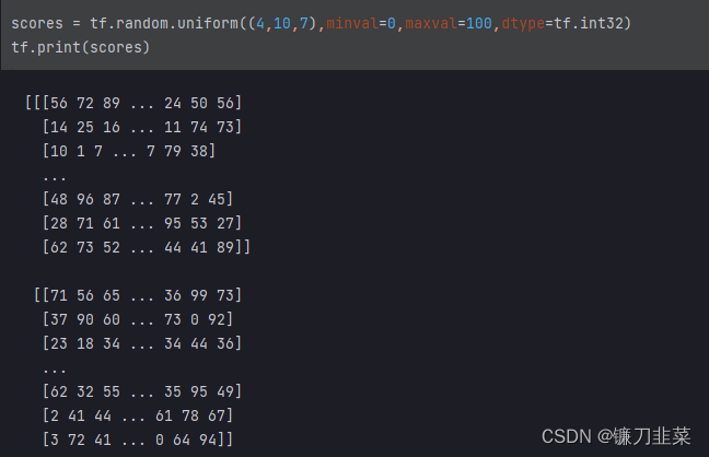
抽取每个班级第0个学生，第5个学生，第9个学生的第1门课程，第3门课程，第6门课程成绩：

q = tf.gather(tf.gather(scores,[0,5,9],axis=1),[1,3,6],axis=2)
tf.print(q)

抽取第0个班级第0个学生，第2个班级的第4个学生，第3个班级的第6个学生的全部成绩：

# indices的长度为采样样本的个数，每个元素为采样位置的坐标
s = tf.gather_nd(scores, indices=[(0,0),(2,4),(3,6)])
tf.print(s)
'''
[[56 72 89 ... 24 50 56]
 [25 69 37 ... 71 60 16]
 [31 93 50 ... 41 71 59]]
'''

以上tf.gather和tf.gather_nd的功能也可以用tf.boolean_mask来实现。抽取每个班级第0个学生，第5个学生，第9个学生的全部成绩：

p = tf.boolean_mask(scores, [True,False,False,False,False,True,False,False,False,True],axis=1)
tf.print(p)

'''
[[[56 72 89 ... 24 50 56]
  [23 96 38 ... 63 54 41]
  [62 73 52 ... 44 41 89]]

 [[71 56 65 ... 36 99 73]
  [85 81 30 ... 14 80 3]
  [3 72 41 ... 0 64 94]]

 [[1 25 83 ... 2 20 6]
  [61 88 85 ... 42 3 45]
  [69 85 4 ... 60 27 46]]

 [[41 38 86 ... 57 94 72]
  [17 79 35 ... 73 29 92]
  [91 66 55 ... 71 29 9]]]
'''

抽取第0个班级第0个学生，第2个班级的第4个学生，第3个班级的第6个学生的全部成绩：

s = tf.boolean_mask(scores,
    [[True,False,False,False,False,False,False,False,False,False],
     [False,False,False,False,False,False,False,False,False,False],
     [False,False,False,False,True,False,False,False,False,False],
     [False,False,False,False,False,False,True,False,False,False]])
tf.print(s)
'''
[[56 72 89 ... 24 50 56]
 [25 69 37 ... 71 60 16]
 [31 93 50 ... 41 71 59]]
'''

利用tf.boolean_mask可以实现布尔索引:

# 找到矩阵中小于0的元素
c = tf.constant([[-1,1,-1],[2,2,-2],[3,-3,3]],dtype=tf.float32)
tf.print(c,"\n")

tf.print(tf.boolean_mask(c,c<0),'\n')
tf.print(c[c<0]) # 布尔索引，为boolean_mask的语法糖形式

'''
[[-1 1 -1]
 [2 2 -2]
 [3 -3 3]] 

[-1 -1 -2 -3] 

[-1 -1 -2 -3]
'''

以上这些方法仅能提取张量的部分元素值，但不能更改张量的部分元素值得到新的张量。

如果要通过修改张量的部分元素值得到新的张量，可以使用tf.where和tf.scatter_nd。

tf.where可以理解为if的张量版本，此外它还可以用于找到满足条件的所有元素的位置坐标。
tf.scatter_nd的作用和tf.gather_nd有些相反，tf.gather_nd用于收集张量的给定位置的元素，而tf.scatter_nd可以将某些值插入到一个给定shape的全0的张量的指定位置处。

找到张量中小于0的元素，将其换成np.nan得到新的张量：

# tf.where和np.where作用类似，可以理解为if的张量版本
c = tf.constant([[-1, 1, -1],[2, 2, -2],[3, -3, 3]], dtype=tf.float32)
d = tf.where(c<0, tf.fill(c.shape, np.nan), c)
d
'''
<tf.Tensor: shape=(3, 3), dtype=float32, numpy=
array([[nan,  1., nan],
       [ 2.,  2., nan],
       [ 3., nan,  3.]], dtype=float32)>
'''

如果where只有一个参数，将返回所有满足条件的位置坐标：

indices = tf.where(c<0)
indices
'''
<tf.Tensor: shape=(4, 2), dtype=int64, numpy=
array([[0, 0],
       [0, 2],
       [1, 2],
       [2, 1]], dtype=int64)>
'''

将张量的第[0, 0]和[2, 1]两个位置元素替换为0得到新的张量：

d = c - tf.scatter_nd([[0,0],[2,1]],[c[0,0],c[2,1]],c.shape)
d
'''
<tf.Tensor: shape=(3, 3), dtype=float32, numpy=
array([[ 0.,  1., -1.],
       [ 2.,  2., -2.],
       [ 3.,  0.,  3.]], dtype=float32)>
'''

scatter_nd的作用和gather_nd有些相反，可以将某些值插入到一个给定shape的全0的张量的指定位置处。

indices = tf.where(c<0)
tf.scatter_nd(indices,tf.gather_nd(c,indices),c.shape)
'''
<tf.Tensor: shape=(3, 3), dtype=float32, numpy=
array([[-1.,  0., -1.],
       [ 0.,  0., -2.],
       [ 0., -3.,  0.]], dtype=float32)>
'''

维度变换

维度变换相关函数主要有tf.reshape, tf.squeeze, tf.expand_dims, tf.transpose。

tf.reshape可以改变张量的形状。
tf.squeeze可以减少维度。
tf.expand_dims可以增加维度。
tf.transpose可以交换维度。

tf.reshape可以改变张量的形状，但是其本质上不会改变张量元素的存储顺序，所以，该操作实际上非常迅速，并且是可逆的。

a = tf.random.uniform(shape=[1,3,3,2], minval=0, maxval=255, dtype=tf.int32)
tf.print(a.shape)
tf.print(a)
'''
TensorShape([1, 3, 3, 2])
[[[[61 192]
   [123 134]
   [8 141]]

  [[223 19]
   [180 0]
   [236 153]]

  [[154 0]
   [146 15]
   [120 201]]]]
'''

改成（3，6）形状的张量：

b = tf.reshape(a,[3,6])
tf.print(b.shape)
tf.print(b)
'''
TensorShape([3, 6])
[[61 192 123 134 8 141]
 [223 19 180 0 236 153]
 [154 0 146 15 120 201]]
'''

改回 [1,3,3,2] 形状的张量:

c = tf.reshape(b,[1,3,3,2])
tf.print(c)

如果张量在某个维度上只有一个元素，利用tf.squeeze可以消除这个维度，和tf.reshape相似，它本质上不会改变张量元素的存储顺序。
张量的各个元素在内存中是线性存储的，其一般规律是，同一层级中的相邻元素的物理地址也相邻。

s = tf.squeeze(a)
tf.print(s.shape)
tf.print(s)
'''
TensorShape([3, 3, 2])
[[[61 192]
  [123 134]
  [8 141]]

 [[223 19]
  [180 0]
  [236 153]]

 [[154 0]
  [146 15]
  [120 201]]]
'''

在第0维插入长度为1的一个维度：

d = tf.expand_dims(s, axis=0)
d
'''
<tf.Tensor: shape=(1, 3, 3, 2), dtype=int32, numpy=
array([[[[ 61, 192],
         [123, 134],
         [  8, 141]],

        [[223,  19],
         [180,   0],
         [236, 153]],

        [[154,   0],
         [146,  15],
         [120, 201]]]])>
'''

tf.transpose可以交换张量的维度，与tf.reshape不同，它会改变张量元素的存储顺序。tf.transpose常用于图片存储格式的变换上。

# Batch,Height,Width,Channel
a = tf.random.uniform(shape=[100,600,600,4],minval=0,maxval=255,dtype=tf.int32)
tf.print(a.shape)

# 转换成 Channel,Height,Width,Batch
s= tf.transpose(a,perm=[3,1,2,0])
tf.print(s.shape)
'''
TensorShape([100, 600, 600, 4])
TensorShape([4, 600, 600, 100])
'''

分割与合并

和numpy类似，可以用tf.concat和tf.stack方法对多个张量进行合并，可以用tf.split方法把一个张量分割成多个张量。
注意：tf.concat和tf.stack有略微的区别，tf.concat是连接，不会增加维度，而tf.stack是堆叠，会增加维度。

a = tf.constant([[1.0,2.0],[3.0,4.0]])
b = tf.constant([[5.0,6.0],[7.0,8.0]])
c = tf.constant([[9.0,10.0],[11.0,12.0]])

tf.concat([a,b,c],axis = 0)
'''
<tf.Tensor: shape=(6, 2), dtype=float32, numpy=
array([[ 1.,  2.],
       [ 3.,  4.],
       [ 5.,  6.],
       [ 7.,  8.],
       [ 9., 10.],
       [11., 12.]], dtype=float32)>
'''
tf.concat([a, b, c],axis = 1)
'''
<tf.Tensor: shape=(2, 6), dtype=float32, numpy=
array([[ 1.,  2.,  5.,  6.,  9., 10.],
       [ 3.,  4.,  7.,  8., 11., 12.]], dtype=float32)>
'''
tf.stack([a,b,c])
'''
<tf.Tensor: shape=(3, 2, 2), dtype=float32, numpy=
array([[[ 1.,  2.],
        [ 3.,  4.]],

       [[ 5.,  6.],
        [ 7.,  8.]],

       [[ 9., 10.],
        [11., 12.]]], dtype=float32)>
'''
tf.stack([a,b,c], axis=1)
'''
<tf.Tensor: shape=(2, 3, 2), dtype=float32, numpy=
array([[[ 1.,  2.],
        [ 5.,  6.],
        [ 9., 10.]],

       [[ 3.,  4.],
        [ 7.,  8.],
        [11., 12.]]], dtype=float32)>
'''

tf.split是tf.concat的逆运算，可以指定分割份数平均分割，也可以通过指定每份的记录数量进行分割。

#tf.split(value,num_or_size_splits,axis)
tf.split(c, 3, axis = 0)  #指定分割份数，平均分割

'''
[<tf.Tensor: shape=(2, 2), dtype=float32, numpy=
 array([[1., 2.],
        [3., 4.]], dtype=float32)>,
 <tf.Tensor: shape=(2, 2), dtype=float32, numpy=
 array([[5., 6.],
        [7., 8.]], dtype=float32)>,
 <tf.Tensor: shape=(2, 2), dtype=float32, numpy=
 array([[ 9., 10.],
        [11., 12.]], dtype=float32)>]
'''
tf.split(c,[2, 2, 2], axis = 0) #指定每份的记录数量
'''
[<tf.Tensor: shape=(2, 2), dtype=float32, numpy=
 array([[1., 2.],
        [3., 4.]], dtype=float32)>,
 <tf.Tensor: shape=(2, 2), dtype=float32, numpy=
 array([[5., 6.],
        [7., 8.]], dtype=float32)>,
 <tf.Tensor: shape=(2, 2), dtype=float32, numpy=
 array([[ 9., 10.],
        [11., 12.]], dtype=float32)>]
'''

Tensorflow中的数学运算

张量的数学运算符可以分为标量运算符、向量运算符、以及矩阵运算符。

标量运算

加减乘除乘方，以及三角函数，指数，对数等常见函数，逻辑比较运算符等都是标量运算符。
标量运算符的特点是对张量实施逐元素运算。
有些标量运算符对常用的数学运算符进行了重载。并且支持类似numpy的广播特性。
许多标量运算符都在tf.math模块下。

import tensorflow as tf 
import numpy as np

标量运算：

a = tf.constant([[1.0,2],[-3,4.0]])
b = tf.constant([[5.0,6],[7.0,8.0]])
a + b  #运算符重载
'''
<tf.Tensor: shape=(2, 2), dtype=float32, numpy=
array([[ 6.,  8.],
       [ 4., 12.]], dtype=float32)>
'''
a-b 
'''
<tf.Tensor: shape=(2, 2), dtype=float32, numpy=
array([[ -4.,  -4.],
       [-10.,  -4.]], dtype=float32)>
'''
a*b
'''
<tf.Tensor: shape=(2, 2), dtype=float32, numpy=
array([[  5.,  12.],
       [-21.,  32.]], dtype=float32)>
'''
a/b
'''
<tf.Tensor: shape=(2, 2), dtype=float32, numpy=
array([[ 0.2       ,  0.33333334],
       [-0.42857143,  0.5       ]], dtype=float32)>
'''
a**2
'''
<tf.Tensor: shape=(2, 2), dtype=float32, numpy=
array([[ 1.,  4.],
       [ 9., 16.]], dtype=float32)>
'''
a**(0.5)
'''
<tf.Tensor: shape=(2, 2), dtype=float32, numpy=
array([[1.       , 1.4142135],
       [      nan, 2.       ]], dtype=float32)>
'''
a%3 #mod的运算符重载，等价于m = tf.math.mod(a,3)
'''
<tf.Tensor: shape=(3,), dtype=int32, numpy=array([1, 2, 0], dtype=int32)>
'''
a//3 #地板除法
'''
<tf.Tensor: shape=(2, 2), dtype=float32, numpy=
array([[ 0.,  0.],
       [-1.,  1.]], dtype=float32)>
'''
(a>=2) # 逻辑运算符
'''
<tf.Tensor: shape=(2, 2), dtype=bool, numpy=
array([[False,  True],
       [False,  True]])>
'''
(a>=2)&(a<=3)
'''
<tf.Tensor: shape=(2, 2), dtype=bool, numpy=
array([[False,  True],
       [False, False]])>
'''
(a>=2)|(a<=3)
'''
<tf.Tensor: shape=(2, 2), dtype=bool, numpy=
array([[ True,  True],
       [ True,  True]])>
'''
a==5 #tf.equal(a,5)
'''
<tf.Tensor: shape=(3,), dtype=bool, numpy=array([False, False, False])>
'''
tf.sqrt(a)
'''
<tf.Tensor: shape=(2, 2), dtype=float32, numpy=
array([[1.       , 1.4142135],
       [      nan, 2.       ]], dtype=float32)>
'''
a = tf.constant([1.0,8.0])
b = tf.constant([5.0,6.0])
c = tf.constant([6.0,7.0])
tf.add_n([a,b,c]) # 元素逐位置相加
'''
<tf.Tensor: shape=(2,), dtype=float32, numpy=array([12., 21.], dtype=float32)>
'''
tf.print(tf.maximum(a,b))
'''
[5 8]
'''
tf.print(tf.minimum(a,b))
'''
[1 6]
'''
x = tf.constant([2.6,-2.7])

tf.print(tf.math.round(x)) #保留整数部分，四舍五入
tf.print(tf.math.floor(x)) #保留整数部分，向下归整
tf.print(tf.math.ceil(x))  #保留整数部分，向上归整
'''
[3 -3]
[2 -3]
[3 -2]
'''

# 幅值裁剪
x = tf.constant([0.9,-0.8,100.0,-20.0,0.7])
y = tf.clip_by_value(x,clip_value_min=-1,clip_value_max=1)
z = tf.clip_by_norm(x,clip_norm = 3)
tf.print(y)
tf.print(z)
'''
[0.9 -0.8 1 -1 0.7]
[0.0264732055 -0.0235317405 2.94146752 -0.588293493 0.0205902718]
'''

向量运算

向量运算符只在一个特定轴上运算，将一个向量映射到一个标量或者另外一个向量。许多向量运算符都以reduce开头。
（1）向量reduce

a = tf.range(1, 10)
tf.print(a)
tf.print(tf.reduce_sum(a)) 
tf.print(tf.reduce_mean(a))
tf.print(tf.reduce_max(a))
tf.print(tf.reduce_min(a))
tf.print(tf.reduce_prod(a))
'''
[1 2 3 ... 7 8 9]
45
5
9
1
362880
'''

（2）张量指定维度进行reduce

b = tf.reshape(a, (3, 3))
tf.print(b)
tf.print(tf.reduce_sum(b, axis=1, keepdims=True))
tf.print(tf.reduce_sum(b, axis=0, keepdims=True))
'''
[[1 2 3]
 [4 5 6]
 [7 8 9]]
[[6]
 [15]
 [24]]
[[12 15 18]]
'''

（3）bool类型的reduce

p = tf.constant([True,False,False])
q = tf.constant([False,False,True])
tf.print(tf.reduce_all(p)) # 0
tf.print(tf.reduce_any(q)) # 1

（4）利用tf.foldr实现tf.reduce_sum

s = tf.foldr(lambda a,b:a+b,tf.range(10)) 
tf.print(s) # 45

（5）cum扫描累积

a = tf.range(1,10)
tf.print(tf.math.cumsum(a))
tf.print(tf.math.cumprod(a))
'''
[1 3 6 ... 28 36 45]
[1 2 6 ... 5040 40320 362880]
'''

（6）arg最大最小值索引

a = tf.range(1,10)
tf.print(tf.argmax(a)) # 8
tf.print(tf.argmin(a)) # 0

（7）tf.math.top_k可以用于对张量排序

a = tf.constant([1,3,7,5,4,8])

values,indices = tf.math.top_k(a,3,sorted=True)
tf.print(values)
tf.print(indices)

#利用tf.math.top_k可以在TensorFlow中实现KNN算法
'''
[8 7 5]
[5 2 3]
'''

矩阵运算

矩阵必须是二维的。类似tf.constant([1,2,3])这样的不是矩阵。
矩阵运算包括：矩阵乘法，矩阵转置，矩阵逆，矩阵求迹，矩阵范数，矩阵行列式，矩阵求特征值，矩阵分解等运算。
除了一些常用的运算外，大部分和矩阵有关的运算都在tf.linalg子包中。

# 矩阵乘法
a = tf.constant([[1,2],[3,4]])
b = tf.constant([[2,0],[0,2]])
a@b  #等价于tf.matmul(a,b)
'''
<tf.Tensor: shape=(2, 2), dtype=int32, numpy=
array([[2, 4],
       [6, 8]], dtype=int32)>
'''
# 矩阵转置
a = tf.constant([[1,2],[3,4]])
tf.transpose(a)
'''
<tf.Tensor: shape=(2, 2), dtype=int32, numpy=
array([[1, 3],
       [2, 4]], dtype=int32)>
'''
# 矩阵逆，必须为tf.float32或tf.double类型
a = tf.constant([[1.0,2],[3,4]],dtype = tf.float32)
tf.linalg.inv(a)
'''
<tf.Tensor: shape=(2, 2), dtype=float32, numpy=
array([[-2.0000002 ,  1.0000001 ],
       [ 1.5000001 , -0.50000006]], dtype=float32)>
'''
# 矩阵求trace
a = tf.constant([[1.0,2],[3,4]],dtype = tf.float32)
tf.linalg.trace(a)
'''
<tf.Tensor: shape=(), dtype=float32, numpy=5.0>
'''
# 矩阵求范数
a = tf.constant([[1.0,2],[3,4]])
tf.linalg.norm(a)
'''
<tf.Tensor: shape=(), dtype=float32, numpy=5.477226>
'''
# 矩阵行列式
a = tf.constant([[1.0,2],[3,4]])
tf.linalg.det(a)
'''
<tf.Tensor: shape=(), dtype=float32, numpy=-2.0>
'''
# 矩阵特征值
a = tf.constant([[1.0,2],[-5,4]])
tf.linalg.eigvals(a)
'''
<tf.Tensor: shape=(2,), dtype=complex64, numpy=array([2.4999995+2.7838817j, 2.5      -2.783882j ], dtype=complex64)>
'''

矩阵QR分解, 将一个方阵分解为一个正交矩阵q和上三角矩阵r：

# QR分解实际上是对矩阵a实施Schmidt正交化得到q

a = tf.constant([[1.0, 2.0], [3.0, 4.0]], dtype=tf.float32)
q, r = tf.linalg.qr(a)
tf.print(q)
tf.print(r)
tf.print(q @ r)
'''
[[-0.316227794 -0.948683321]
 [-0.948683321 0.316227734]]
[[-3.1622777 -4.4271884]
 [0 -0.632455349]]
[[1.00000012 1.99999976]
 [3 4]]
'''

矩阵SVD分解:

#svd分解可以将任意一个矩阵分解为一个正交矩阵u,一个对角阵s和一个正交矩阵v.t()的乘积
#svd常用于矩阵压缩和降维

a  = tf.constant([[1.0,2.0],[3.0,4.0],[5.0,6.0]], dtype = tf.float32)
s,u,v = tf.linalg.svd(a)
tf.print(u,"\n")
tf.print(s,"\n")
tf.print(v,"\n")
tf.print(u@tf.linalg.diag(s)@tf.transpose(v))

#利用svd分解可以在TensorFlow中实现主成分分析降维
'''
[[-0.229847893 0.883461297]
 [-0.524744868 0.240781844]
 [-0.819642 -0.401895821]] 

[9.52551937 0.514301538] 

[[-0.619629383 -0.784894526]
 [-0.784894526 0.619629383]] 

[[1.00000024 2.00000238]
 [3.00000024 4.00000143]
 [5.00000048 6.00000143]]
'''

广播机制

TensorFlow的广播规则和numpy是一样的:

如果张量的维度不同，将维度较小的张量进行扩展，直到两个张量的维度都一样。
如果两个张量在某个维度上的长度是相同的，或者其中一个张量在该维度上的长度为1，那么我们就说这两个张量在该维度上是相容的。
如果两个张量在所有维度上都是相容的，它们就能使用广播。
广播之后，每个维度的长度将取两个张量在该维度长度的较大值。
在任何一个维度上，如果一个张量的长度为1，另一个张量长度大于1，那么在该维度上，就好像是对第一个张量进行了复制。

tf.broadcast_to以显式的方式按照广播机制扩展张量的维度。

a = tf.constant([1,2,3])
b = tf.constant([[0,0,0],[1,1,1],[2,2,2]])
b + a  #等价于 b + tf.broadcast_to(a,b.shape)
'''
<tf.Tensor: shape=(3, 3), dtype=int32, numpy=
array([[1, 2, 3],
       [2, 3, 4],
       [3, 4, 5]], dtype=int32)>
'''
tf.broadcast_to(a,b.shape)
'''
<tf.Tensor: shape=(3, 3), dtype=int32, numpy=
array([[1, 2, 3],
       [1, 2, 3],
       [1, 2, 3]], dtype=int32)>
'''

计算广播后计算结果的形状，静态形状，TensorShape类型参数:

tf.broadcast_static_shape(a.shape,b.shape)
'''
TensorShape([3, 3])
'''

计算广播后计算结果的形状，动态形状，Tensor类型参数

c = tf.constant([1,2,3])
d = tf.constant([[1],[2],[3]])
tf.broadcast_dynamic_shape(tf.shape(c),tf.shape(d))
'''
<tf.Tensor: shape=(2,), dtype=int32, numpy=array([3, 3], dtype=int32)>
'''

广播效果:

c+d #等价于 tf.broadcast_to(c,[3,3]) + tf.broadcast_to(d,[3,3])
'''
<tf.Tensor: shape=(3, 3), dtype=int32, numpy=
array([[2, 3, 4],
       [3, 4, 5],
       [4, 5, 6]], dtype=int32)>
'''

Tensorflow中的AutoGraph计算图

AutoGraph的使用规范

目前，有三种计算图的构建方式：静态计算图，动态计算图，以及Autograph。TensorFlow 2.0主要使用的是动态计算图和Autograph。

动态计算图易于调试，编码效率较高，但执行效率偏低。
静态计算图执行效率很高，但较难调试。
Autograph机制可以将动态图转换成静态计算图，同时具有执行效率和编码效率的优势。

当然Autograph机制能够转换的代码并不是没有任何约束的，有一些编码规范需要遵循，否则可能会转换失败或者不符合预期。接下来介绍Autograph的编码规范和Autograph转换成静态图的原理，并介绍使用tf.Module来更好地构建Autograph。

Autograph编码规范

被@tf.function修饰的函数应尽可能使用TensorFlow中的函数而不是Python中的其他函数。例如使用tf.print而不是print，使用tf.range而不是range，使用tf.constant(True)而不是True.
避免在@tf.function修饰的函数内部定义tf.Variable.
被@tf.function修饰的函数不可修改该函数外部的Python列表或字典等数据结构变量。

Autograph编码示例

被@tf.function修饰的函数应尽量使用TensorFlow中的函数而不是Python中的其他函数。

import numpy as np
import tensorflow as tf

@tf.function
def np_random():
    a = np.random.randn(3,3)
    tf.print(a)

@tf.function
def tf_random():
    a = tf.random.normal((3,3))
    tf.print(a)

np_random每次执行都是一样的结果：

np_random()
np_random()
'''
array([[ 0.50224647, -0.15924273,  0.727995  ],
       [-0.37840825, -1.00053087, -0.78702307],
       [ 1.26153662,  1.64081248, -1.57451626]])
array([[ 0.50224647, -0.15924273,  0.727995  ],
       [-0.37840825, -1.00053087, -0.78702307],
       [ 1.26153662,  1.64081248, -1.57451626]])
'''

tf_random每次执行都会有重新生成随机数:

tf_random()
tf_random()
'''
[[-0.302002043 1.99549484 -1.43466115]
 [-2.59828162 0.0505513214 -0.533689559]
 [-0.0854836 1.53205907 0.352520168]]
[[-1.49828815 1.54806888 1.26572335]
 [2.20143676 -0.256682128 -0.273425788]
 [-0.0966404602 -0.248796791 -0.629100084]]
'''

避免在@tf.function修饰的函数内部定义tf.Variable.

x = tf.Variable(1.0, dtype=tf.float32)


@tf.function
def outer_var():
    x.assign_add(1.0)
    tf.print(x)
    return (x)


outer_var() # 2
outer_var() # 3

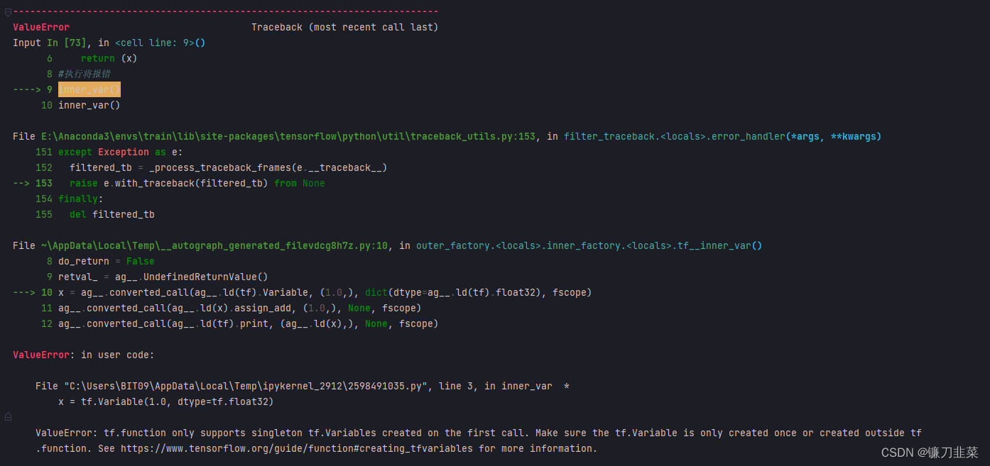
如果在@tf.function修饰的函数内部定义tf.Variable，则将报错：

@tf.function
def inner_var():
    x = tf.Variable(1.0, dtype=tf.float32)
    x.assign_add(1.0)
    tf.print(x)
    return x


#执行将报错
inner_var()
inner_var()

报错信息

被@tf.function修饰的函数不可修改该函数外部的Python列表或字典等结构类型变量。

tensor_list = []


#@tf.function #加上这一行切换成Autograph结果将不符合预期！！！
def append_tensor(x):
    tensor_list.append(x)
    return tensor_list


append_tensor(tf.constant(5.0))
append_tensor(tf.constant(6.0))
print(tensor_list)
'''
[<tf.Tensor: shape=(), dtype=float32, numpy=5.0>, <tf.Tensor: shape=(), dtype=float32, numpy=6.0>]
'''

tensor_list = []

@tf.function #加上这一行切换成Autograph结果将不符合预期！！！
def append_tensor(x):
    tensor_list.append(x)
    return tensor_list


append_tensor(tf.constant(5.0))
append_tensor(tf.constant(6.0))
print(tensor_list)
'''
[<tf.Tensor 'x:0' shape=() dtype=float32>]
'''

AutoGraph的机制原理

当使用@tf.function装饰一个函数的时候，后面到底发生了什么呢？

import tensorflow as tf
import numpy as np 

@tf.function(autograph=True)
def myadd(a,b):
    for i in tf.range(3):
        tf.print(i)
    c = a+b
    print("tracing")
    return c

当我们第一次调用这个被@tf.function装饰的函数时，后面到底发生了什么？

myadd(tf.constant('hello'), tf.constant(' world'))
'''
tracing
0
1
2
'''

发生了2件事情：
①第一件事情是创建计算图，即创建一个静态计算图，跟踪执行一遍函数体中的Python代码，确定各个变量的Tensor类型，并根据执行顺序将算子添加到计算图中。在这个过程中，如果开启了autograph=True(默认开启)，会将Python控制流转换成TensorFlow图内控制流。主要是将if语句转换成 tf.cond算子表达，将while和for循环语句转换成tf.while_loop算子表达，并在必要的时候添加tf.control_dependencies指定执行顺序依赖关系。
②第二件事情是执行计算图。因此先看到的是第一个步骤的结果：即Python调用标准输出流打印"tracing"语句。然后看到第二个步骤的结果：TensorFlow调用标准输出流打印0,1,2。

当我们再次用相同的输入参数类型调用这个被@tf.function装饰的函数时，后面到底发生了什么？

0
1
2

只会发生一件事情，那就是上面步骤的第二步，执行计算图。所以这一次没有看到打印"tracing"的结果。

当再次用不同的的输入参数类型调用这个被@tf.function装饰的函数时，后面到底发生了什么？

myadd(tf.constant(1),tf.constant(2))
'''
tracing
0
1
2
'''

由于输入参数的类型已经发生变化，已经创建的计算图不能够再次使用。所以需要重新做2件事情：创建新的计算图、执行计算图。

需要注意的是，如果调用被@tf.function装饰的函数时输入的参数不是Tensor类型，则每次都会重新创建计算图。

myadd("hello","world")
myadd("good","morning")
'''
tracing
0
1
2
tracing
0
1
2
'''

因此，一般建议调用@tf.function时应传入Tensor类型。

AutoGraph的编码规范再理解

被@tf.function修饰的函数应尽量使用TensorFlow中的函数而不是Python中的其他函数。例如使用tf.print而不是print。
原因：Python中的函数仅仅会在跟踪执行函数以创建静态图的阶段使用，普通python函数是无法嵌入到静态计算图中的，所以在计算图构建好之后再次调用的时候，这些python函数并没有被计算，而Tensorflow中的函数则可以嵌入到计算图中。所以使用普通的Python函数会导致被@tf.function修饰前(eager执行)和被@tf.function修饰后(静态图执行)的输出不一致。
避免在@tf.function修饰的函数内部定义tf.Variable.
原因：如果函数内部定义了tf.Variable,那么在(eager执行)时，这种创建tf.Variable的行为在每次函数调用时候都会发生。但是在静态图执行时，这种创建tf.Variable的行为只会发生在第一步跟踪Python代码逻辑创建计算图时，这会导致被@tf.function修饰前(eager执行)和被@tf.function修饰后(静态图执行)的输出不一致。实际上，TensorFlow在这种情况下一般会报错。
被@tf.function修饰的函数不可修改该函数外部的Python列表或字典等数据结构变量。
原因：静态计算图是被编译成C++代码在TensorFlow内核中执行的。Python中的列表和字典等数据结构变量是无法嵌入到计算图中，它们仅仅能够在创建计算图时被读取，因此在执行计算图时是无法修改Python中的列表或字典这样的数据结构变量的。

Tensorflow中的AutoGraph与tf.Module

前面在介绍Autograph的编码规范时提到构建Autograph时应该避免在@tf.function修饰的函数内部定义tf.Variable。但是如果在函数外部定义tf.Variable的话，又会显得这个函数有外部变量依赖，封装不够完美。

一种简单的思路是定义一个类，并将相关的tf.Variable创建放在类的初始化方法中，而将函数的逻辑放在其他方法中。
另一种方法是TensorFlow提供了一个基类tf.Module，通过继承它构建子类，可以非常方便地管理变量，还可以非常方便地管理它引用的其它Module，最重要的是，能够利用tf.saved_model保存模型并实现跨平台部署使用。

实际上，tf.keras.models.Model,tf.keras.layers.Layer 都是继承自tf.Module的，提供了方便的变量管理和所引用的子模块管理的功能。因此，利用tf.Module提供的封装，再结合TensoFlow丰富的低阶API，就能够基于TensorFlow开发任意机器学习模型(而非仅仅是神经网络模型)，并实现跨平台部署使用。

应用tf.Module封装Autograph

首先定义一个简单的function：

import tensorflow as tf

x = tf.Variable(1.0, dtype=tf.float32)


#在tf.function中用input_signature限定输入张量的签名类型：shape和dtype
@tf.function(input_signature=[tf.TensorSpec(shape=[], dtype=tf.float32)])
def add_print(a):
    x.assign_add(a)
    tf.print(x)
    return x

输入不符合张量签名的参数将报错：

add_print(tf.constant(3.0)) # 4
#add_print(tf.constant(3)) # 将报错

下面利用tf.Module的子类化将其封装一下：

class DemoModule(tf.Module):
    def __init__(self, init_value=tf.constant(0.0), name=None):
        super(DemoModule, self).__init__(name=name)
        with self.name_scope:  #相当于with tf.name_scope("demo_module")
            self.x = tf.Variable(init_value, dtype=tf.float32, trainable=True)

    @tf.function(input_signature=[tf.TensorSpec(shape=[], dtype=tf.float32)])
    def addprint(self, a):
        with self.name_scope:
            self.x.assign_add(a)
            tf.print(self.x)
            return self.x

demo = DemoModule(init_value=tf.constant(1.0))
result = demo.addprint(tf.constant(5.0)) 
'''
6
'''

查看模块中的全部变量和全部可训练变量:

print(demo.variables)
print(demo.trainable_variables)
'''
(<tf.Variable 'demo_module/Variable:0' shape=() dtype=float32, numpy=6.0>,)
(<tf.Variable 'demo_module/Variable:0' shape=() dtype=float32, numpy=6.0>,)
'''

查看模块中的全部子模块:

demo.submodules

使用tf.saved_model 保存模型，并指定需要跨平台部署的方法:

tf.saved_model.save(demo,"../DemoData/autograph/1",signatures = {"serving_default":demo.addprint})

加载模型:

demo2 = tf.saved_model.load("../DemoData/autograph/1")
demo2.addprint(tf.constant(5.0))

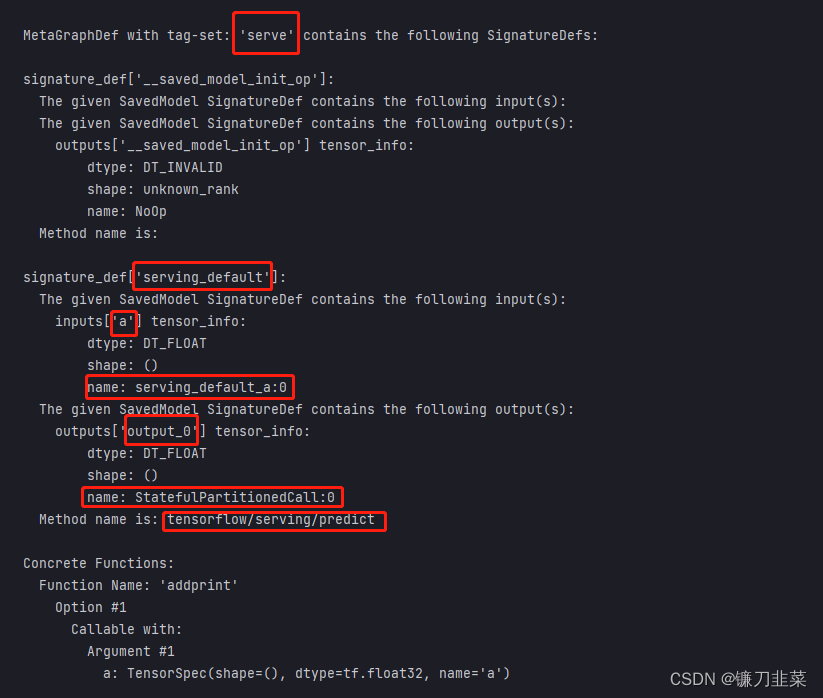
查看模型文件相关信息，红框标出来的输出信息在模型部署和跨平台使用时有可能会用到:

!saved_model_cli show --dir ../DemoData/autograph/1 --all

模型文件信息
除了利用tf.Module的子类化实现封装，也可以通过给tf.Module添加属性的方法进行封装:

mymodule = tf.Module()
mymodule.x = tf.Variable(0.0) # 添加属性

@tf.function(input_signature=[tf.TensorSpec(shape = [], dtype = tf.float32)])
def addprint(a):
    mymodule.x.assign_add(a)
    tf.print(mymodule.x)
    return mymodule.x

mymodule.addprint = addprint
mymodule.addprint(tf.constant(1.0)).numpy() # 1.0
print(mymodule.variables)
'''
(<tf.Variable 'Variable:0' shape=() dtype=float32, numpy=0.0>,)
'''

使用tf.saved_model 保存模型:

tf.saved_model.save(mymodule,"../DemoData/autograph/2",
    signatures = {"serving_default":mymodule.addprint})

#加载模型
mymodule2 = tf.saved_model.load("../DemoData/autograph/2")
mymodule2.addprint(tf.constant(5.0))
'''
INFO:tensorflow:Assets written to: ../DemoData/autograph/2\assets
6
'''

tf.Module和tf.keras.Model, tf.keras.layers.Layer的关系

tf.keras中的模型和层都是继承tf.Module实现的，也具有变量管理和子模块管理功能。

import tensorflow as tf
from tensorflow.keras import models,layers,losses,metrics

print(issubclass(tf.keras.Model,tf.Module)) # True
print(issubclass(tf.keras.layers.Layer,tf.Module)) # True
print(issubclass(tf.keras.Model,tf.keras.layers.Layer)) # True

创建模型：

tf.keras.backend.clear_session() 

model = models.Sequential()

model.add(layers.Dense(4,input_shape = (10,)))
model.add(layers.Dense(2))
model.add(layers.Dense(1))
model.summary()
'''
Model: "sequential"
_________________________________________________________________
 Layer (type)                Output Shape              Param #   
=================================================================
 dense (Dense)               (None, 4)                 44        
                                                                 
 dense_1 (Dense)             (None, 2)                 10        
                                                                 
 dense_2 (Dense)             (None, 1)                 3         
                                                                 
=================================================================
Total params: 57
Trainable params: 57
Non-trainable params: 0
_________________________________________________________________
'''

模型的变量：

model.variables
'''
[<tf.Variable 'dense/kernel:0' shape=(10, 4) dtype=float32, numpy=
 array([[ 0.06851107,  0.6222638 ,  0.18818557, -0.5624115 ],
        [ 0.10263896, -0.5808124 , -0.13333768, -0.01909971],
        [ 0.46239233,  0.56399536,  0.5484568 , -0.41919693],
        [-0.2521158 , -0.44343483, -0.19948038, -0.1928229 ],
        [-0.42875177, -0.24698243,  0.24389917,  0.19735926],
        [-0.3121134 , -0.24455473,  0.01878113, -0.36502132],
        [-0.51711345, -0.26277727,  0.04020506, -0.5468274 ],
        [-0.6365008 ,  0.0702194 , -0.49117038, -0.5075959 ],
        [-0.09411347,  0.37452304, -0.5319024 ,  0.00577706],
        [ 0.53566325,  0.15658683,  0.42216563, -0.4886946 ]],
       dtype=float32)>,
 <tf.Variable 'dense/bias:0' shape=(4,) dtype=float32, numpy=array([0., 0., 0., 0.], dtype=float32)>,
 <tf.Variable 'dense_1/kernel:0' shape=(4, 2) dtype=float32, numpy=
 array([[-9.6579075e-02,  9.5146084e-01],
        [ 9.2552114e-01, -4.6730042e-04],
        [-7.0310831e-02,  3.0072451e-01],
        [-6.3602138e-01, -6.9972920e-01]], dtype=float32)>,
 <tf.Variable 'dense_1/bias:0' shape=(2,) dtype=float32, numpy=array([0., 0.], dtype=float32)>,
 <tf.Variable 'dense_2/kernel:0' shape=(2, 1) dtype=float32, numpy=
 array([[0.8551854],
        [0.5268774]], dtype=float32)>,
 <tf.Variable 'dense_2/bias:0' shape=(1,) dtype=float32, numpy=array([0.], dtype=float32)>]
'''

冻结第0层的变量，使其不可训练:

model.layers[0].trainable = False
model.trainable_variables
'''
[<tf.Variable 'dense_1/kernel:0' shape=(4, 2) dtype=float32, numpy=
 array([[-9.6579075e-02,  9.5146084e-01],
        [ 9.2552114e-01, -4.6730042e-04],
        [-7.0310831e-02,  3.0072451e-01],
        [-6.3602138e-01, -6.9972920e-01]], dtype=float32)>,
 <tf.Variable 'dense_1/bias:0' shape=(2,) dtype=float32, numpy=array([0., 0.], dtype=float32)>,
 <tf.Variable 'dense_2/kernel:0' shape=(2, 1) dtype=float32, numpy=
 array([[0.8551854],
        [0.5268774]], dtype=float32)>,
 <tf.Variable 'dense_2/bias:0' shape=(1,) dtype=float32, numpy=array([0.], dtype=float32)>]
'''

模型的子模块：

model.submodules
'''
(<keras.engine.input_layer.InputLayer at 0x2a6cdd4eca0>,
 <keras.layers.core.dense.Dense at 0x2a59e510280>,
 <keras.layers.core.dense.Dense at 0x2a6cdd4e670>,
 <keras.layers.core.dense.Dense at 0x2a6ce9384c0>)
'''

模型的层：

model.layers
'''
[<keras.layers.core.dense.Dense at 0x2a6cdd4e670>,
 <keras.layers.core.dense.Dense at 0x2a6ce9384c0>,
 <keras.layers.core.dense.Dense at 0x2a59e510280>]
 '''

模型的名称及所属范围：

print(model.name) # sequential
print(model.name_scope()) # sequential/

参考资料

[1] 《Tensorflow：实战Google深度学习框架》
[2] 《30天吃掉那只Tensorflow》