拥抱时代--AI（6）

上一次博文中我们知道了为什么使用逻辑回归，以及逻辑回归简单的工作原理，本次和大家一起分享一个逻辑回归的应用。

案例说明

如下图所示是《spss统计分析》中的一个案例，给出的是学生的几个科目的成绩如下图所示：

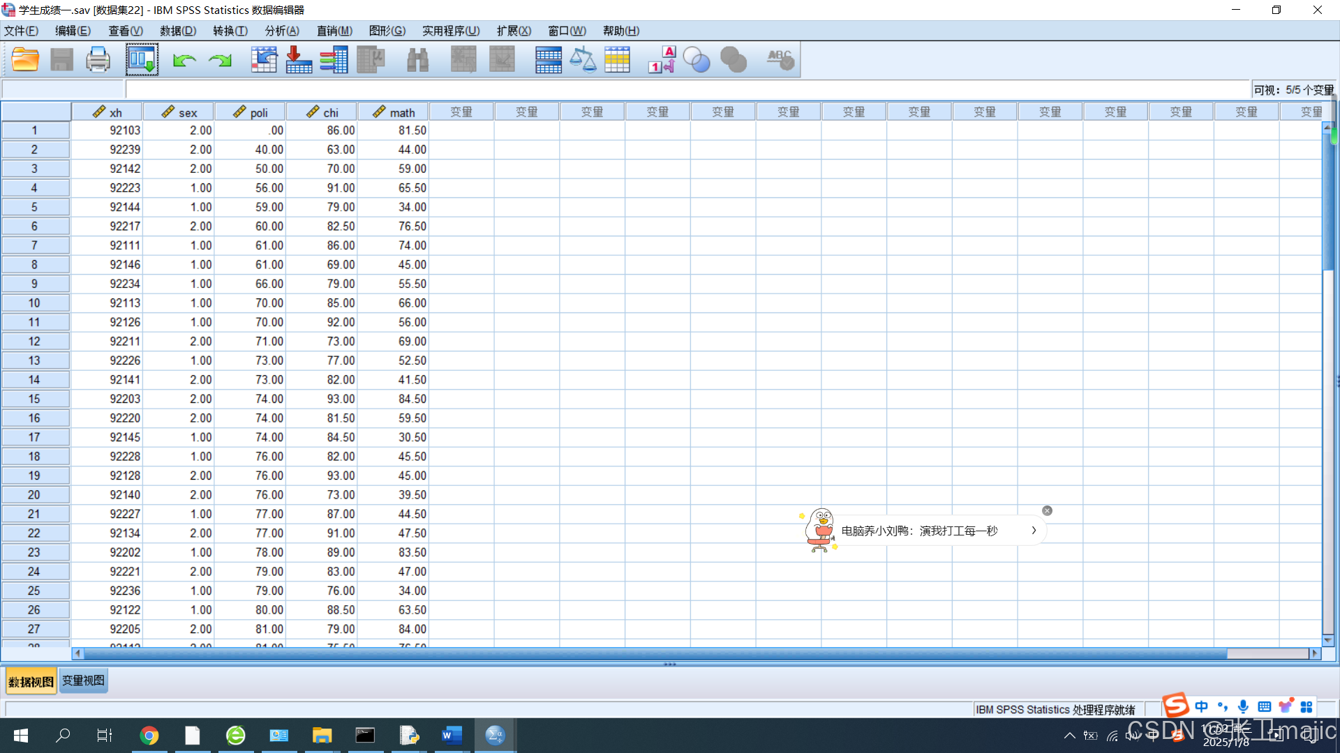
在图中数据为如果成绩有一科不及格则记录为失败，我们计划用poli即政治课和chi（语文？）来作为训练数据，然后通过训练出的模型来预测是否可以通过考试.

1 数据处理

将所有数据存储为cvs，然后通过pandas去读取数据。

from matplotlib import pyplot as plt
import pandas as pd
import numpy as np
import random
from sklearn.linear_model import LinearRegression
from sklearn.metrics import mean_squared_error,r2_score
data=pd.read_csv("e:/1.csv")
poli=data.loc[:,"poli"]
chi=data.loc[:,"chi"]
math=data.loc[:,"math"]
plt.scatter(poli,chi)
plt.show()

得到的直观图形如下：

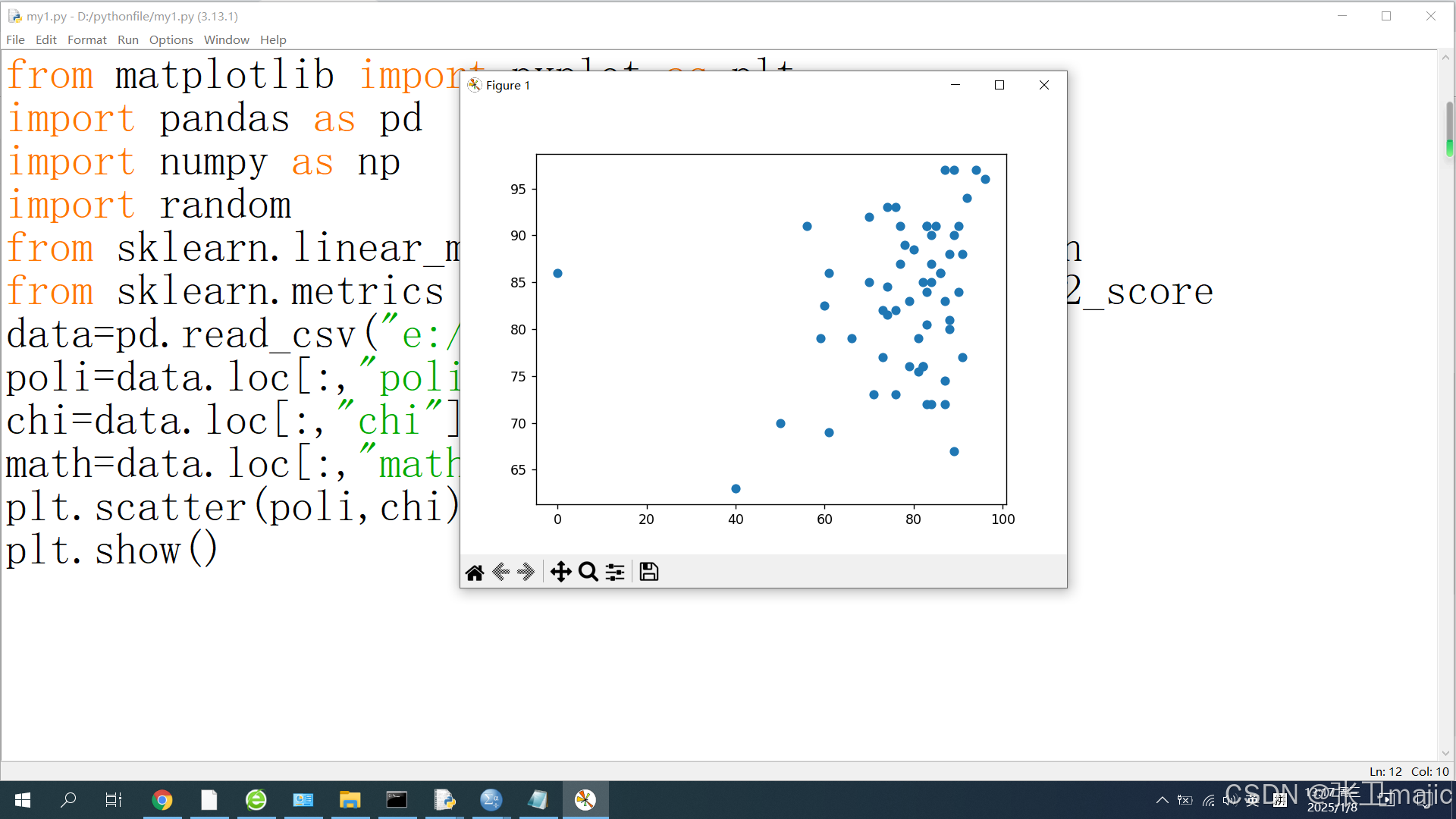
这些点我们并不好直观得到谁通过谁没有通过。我们对数据进行了简要处理，如果有一科低于70分就是失败，其他为通过。在csv中数据如下，各位如果需要可以直接拷贝：

 

xh,gender,poli,chi,math,pass
92103,2,0,86,81.5,0
92239,2,40,63,44,0
92142,2,50,70,59,0
92223,1,56,91,65.5,0
92144,1,59,79,34,0
92217,2,60,82.5,76.5,0
92111,1,61,86,74,0
92146,1,61,69,45,0
92234,1,66,79,55.5,0
92113,1,70,85,66,1
92126,1,70,92,56,1
92211,2,71,73,69,1
92226,1,73,77,52.5,1
92141,2,73,82,41.5,1
92203,2,74,93,84.5,1
92220,2,74,81.5,59.5,1
92145,1,74,84.5,30.5,1
92228,1,76,82,45.5,1
92128,2,76,93,45,1
92140,2,76,73,39.5,1
92227,1,77,87,44.5,1
92134,2,77,91,47.5,1
92202,1,78,89,83.5,1
92221,2,79,83,47,1
92236,1,79,76,34,1
92122,1,80,88.5,63.5,1
92205,2,81,79,84,1
92112,2,81,75.5,76.5,1
92213,1,82,76,65,1
92105,1,82,85,79.5,1
92124,1,82,76,61,1
92207,2,83,91,70.5,1
92215,1,83,80.5,62.5,1
92229,2,83,72,44.5,1
92231,2,83,84,38.5,1
92117,1,83,91,80.5,1
92212,1,84,85,61.5,1
92224,2,84,72,66.5,1
92108,2,84,90,69.5,1
92116,2,84,87,67.5,1
92115,1,85,91,72.5,1
92206,2,86,86,77.5,1
92214,1,86,86,62,1
92216,1,87,74.5,69.5,1
92218,1,87,72,70,1
92225,1,87,83,44.5,1
92127,2,87,97,52,1
92204,2,88,81,87.5,1
92106,2,88,88,78,1
92125,2,88,80,53.5,1
92232,2,89,67,51.5,1
92104,2,89,97,69.5,1
92129,2,89,90,50,1
92209,2,90,91,70.5,1
92120,1,90,84,55,1
92208,1,91,88,63,1
92135,1,91,77,47,1
92110,1,92,94,71,1
92102,1,94,97,86.5,1
92101,2,96,96,87.5,1
对数据进行处理后用如下代码

from matplotlib import pyplot as plt
import pandas as pd
import numpy as np
import random
from sklearn.linear_model import LinearRegression
from sklearn.metrics import mean_squared_error,r2_score
data=pd.read_csv("e:/1.csv")
poli=data.loc[:,"poli"]
chi=data.loc[:,"chi"]
math=data.loc[:,"math"]
fig=plt.figure()
plt.title("political-chinese-score")
plt.xlabel("political")
plt.ylabel("chinese")
mask=data.loc[:,"pass"]==1
print(mask)
tongguo=plt.scatter(poli[mask],chi[mask])
shibai=plt.scatter(poli[~mask],chi[~mask])
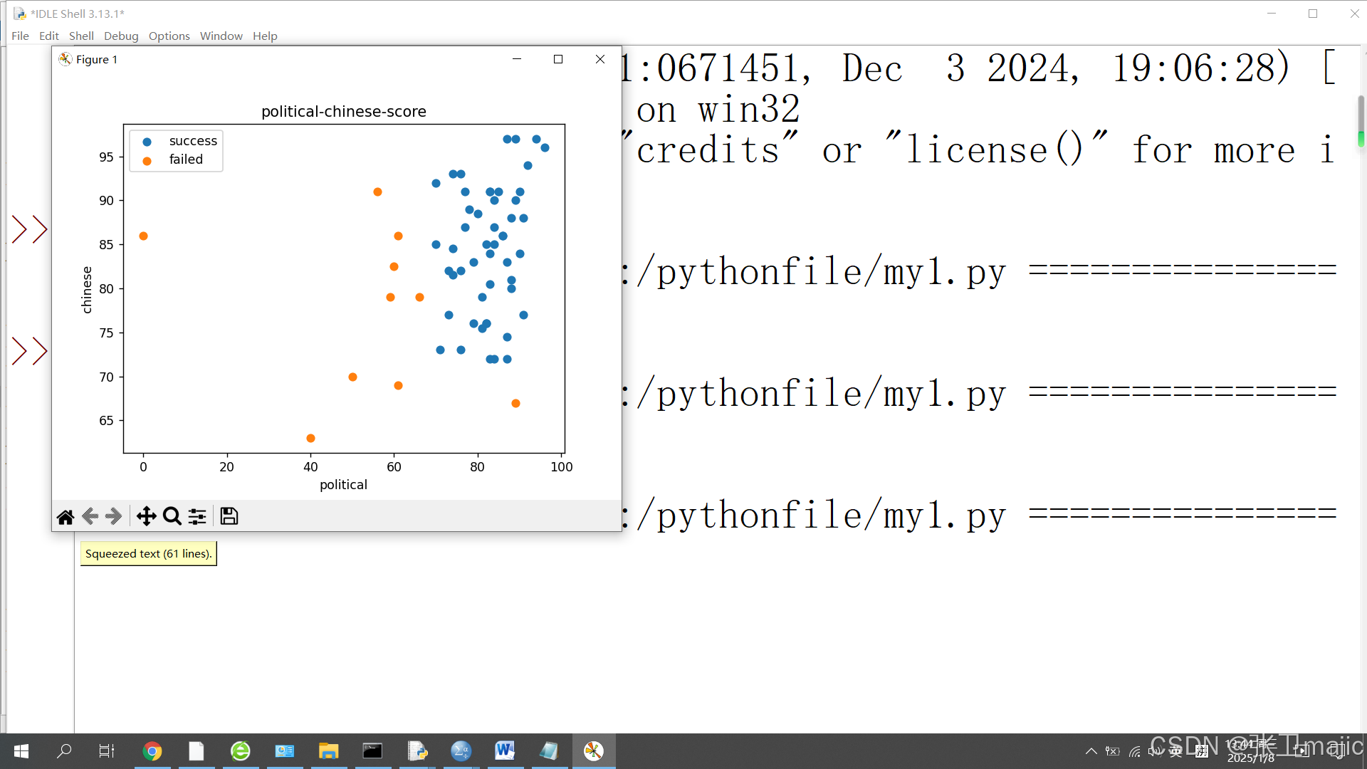
plt.legend((tongguo,shibai),("success","failed"))
plt.show()

此处对通过数据进行了简单处理，并给图形添加了图例，效果如下：

2 回归训练

然后对数据进行模拟训练，代码

from matplotlib import pyplot as plt
import pandas as pd
import numpy as np
import random
from sklearn.linear_model import LinearRegression
from sklearn.linear_model import LogisticRegression
from sklearn.metrics import mean_squared_error,r2_score
data=pd.read_csv("e:/1.csv")
poli=data.loc[:,"poli"]
chi=data.loc[:,"chi"]
math=data.loc[:,"math"]
fig=plt.figure()
plt.title("political-chinese-score")
plt.xlabel("political")
plt.ylabel("chinese")
y=data.loc[:,"pass"]
mask=y==1
print(mask)
tongguo=plt.scatter(poli[mask],chi[mask])
shibai=plt.scatter(poli[~mask],chi[~mask])
plt.legend((tongguo,shibai),("success","failed"))
plt.show()
x=np.array([poli,chi]).transpose()
print(x)
y=np.array(y)
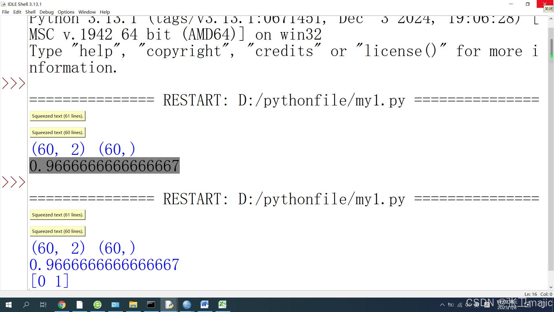
print(x.shape,y.shape)
lr_moxing=LogisticRegression()
lr_moxing.fit(x,y)

可以测试训练的模型，通过代码

from sklearn.metrics import accuracy_score

y_pre=lr_moxing.predict(x)
accuracy=accuracy_score(y,y_pre)
print(accuracy)

得到准确率为0.9666666666666667。

3 预测测试

在此可以通过模型对数据进行预测，如此时一个同学前两门课的成绩分别是70，70，另一个同学是[69,90]其预测：

可以知道第一个同学依模型预测概率不会通过考试，而第二个同学通过考试。到目前所有代码如下可以直接使用：

from matplotlib import pyplot as plt
import pandas as pd
import numpy as np
import random
from sklearn.linear_model import LinearRegression
from sklearn.linear_model import LogisticRegression
from sklearn.metrics import mean_squared_error,r2_score
from sklearn.metrics import accuracy_score
data=pd.read_csv("e:/1.csv")
poli=data.loc[:,"poli"]
chi=data.loc[:,"chi"]
math=data.loc[:,"math"]
fig=plt.figure()
plt.title("political-chinese-score")
plt.xlabel("political")
plt.ylabel("chinese")
y=data.loc[:,"pass"]
mask=y==1
print(mask)
tongguo=plt.scatter(poli[mask],chi[mask])
shibai=plt.scatter(poli[~mask],chi[~mask])
plt.legend((tongguo,shibai),("success","failed"))
plt.show()
x=np.array([poli,chi]).transpose()
print(x)
y=np.array(y)
print(x.shape,y.shape)
lr_moxing=LogisticRegression()
lr_moxing.fit(x,y)
y_pre=lr_moxing.predict(x)
accuracy=accuracy_score(y,y_pre)
print(accuracy)
y_1=lr_moxing.predict([[70,70],[69,90]])
print(y_1)

学习的过程，枯燥而有趣，尝试的过程枯燥而在结果出现的一瞬间又会让有趣的结果稀释前期的无趣，努力吧！

4 边界函数

在上面我们已经通过sklearn对数据进行了简单的模拟，在此想绘制出他们的边界函数。在此次数据的分析过程中x对应两个科目的成绩，可以认为是两个输入参数，他们对应于直角坐标系中图形等下给出，先看其关系式theta0+theta1x1+theta2x2=0

其中theta0，theta1，theta2是我们需要求的参数。通过下面代码

theta0=lr_moxing.intercept_
theta1,theta2=lr_moxing.coef_[0][0],lr_moxing.coef_[0][1]
print(theta0,theta1,theta2)

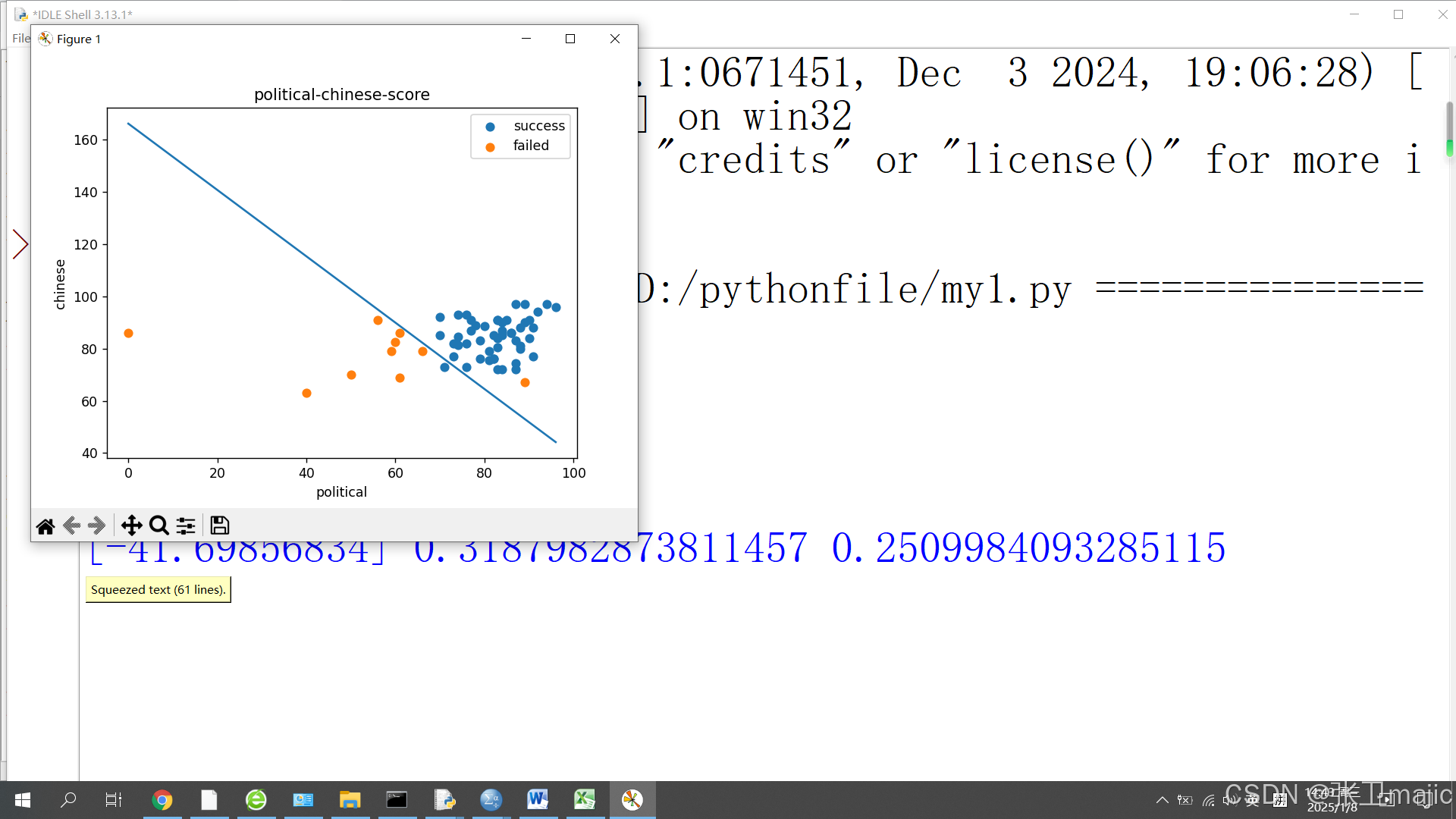
可以得到：-41.69856834 0.3187982873811457 0.2509984093285115

此时即可得到x2=（-theta0-theta1x1）/theta2=41.698-0.31879*x1）/0.250

x1=poli

x2=(-theta0-theata1*x1)/theta2

其对应代码如下：

from matplotlib import pyplot as plt
import pandas as pd
import numpy as np
import random
from sklearn.linear_model import LinearRegression
from sklearn.linear_model import LogisticRegression
from sklearn.metrics import mean_squared_error,r2_score
from sklearn.metrics import accuracy_score
data=pd.read_csv("e:/1.csv")
poli=data.loc[:,"poli"]
chi=data.loc[:,"chi"]
math=data.loc[:,"math"]
fig=plt.figure()
plt.title("political-chinese-score")
plt.xlabel("political")
plt.ylabel("chinese")
y=data.loc[:,"pass"]
mask=y==1
print(mask)
tongguo=plt.scatter(poli[mask],chi[mask])
shibai=plt.scatter(poli[~mask],chi[~mask])
plt.legend((tongguo,shibai),("success","failed"))
#plt.show()
x=np.array([poli,chi]).transpose()
print(x)
y=np.array(y)
print(x.shape,y.shape)
lr_moxing=LogisticRegression()
lr_moxing.fit(x,y)
y_pre=lr_moxing.predict(x)
accuracy=accuracy_score(y,y_pre)
print(accuracy)
y_1=lr_moxing.predict([[70,70],[69,90]])
print(y_1)
theta0=lr_moxing.intercept_
theta1,theta2=lr_moxing.coef_[0][0],lr_moxing.coef_[0][1]
print(theta0,theta1,theta2)
x1=poli
x2=chi
x2_new=(-theta0-theta1*x1)/theta2
print(x2_new)
plt.plot(x1,x2_new)
plt.show()

其中对上述阐述的代码位于代码最下方部分，请大家用心对比。执行效果如下：

当然，如前面所说，这里的边界函数也不一定总是一条直线，如此时边界函数为二阶函数时，假设表达为

theta0+theta1*x1+theta2*x2+theta3*x1^2+theta4*x2^2+theta5*x1*x2=0

则需要构造新的函数

x11=poli*poli

x22=chi*chi

x12=poli*chi

X_new={'x1':poli,'x2':chi,'x11':x11,'x22':x22,'x12':x12}

通过调用

X_new=pd.DataFrame(X_new)
lr_newmodel=LogisticRegression()
lr_newmodel.fit(X_new,y)
y_pre2=lr_newmodel.predict(X_new)
accuracy2=accuracy_score(y,y_pre2)
print(accuracy,accuracy2)
print(lr_newmodel.coef_)

可知准确率比以前更高。0.9666666666666667 1.0，对应的五个系数为：
[[-0.53006379 -0.74892533 -0.02632157 -0.02438616  0.06895139]]

将theta0+theta1*x1+theta2*x2+theta3*x1^2+theta4*x2^2+theta5*x1*x2=0转化为x2和x1的函数即可获得边界函数。具体过程如下图：

由于电脑敲公式台啰嗦了就直接写了一下，后期只要绘制出plot图形即可。这些资料都是我们的亲手资料，大家可以直接拷贝最终代码和数据验证以上所有效果，未来的路上一起加油！

附注 最终所有代码

from  matplotlib import pyplot as plt
import pandas as pd
import numpy as np
import random
from sklearn.linear_model import LinearRegression
from sklearn.linear_model import LogisticRegression
from sklearn.metrics import mean_squared_error,r2_score
from sklearn.metrics import accuracy_score
data=pd.read_csv("e:/1.csv")
poli=data.loc[:,"poli"]
chi=data.loc[:,"chi"]
math=data.loc[:,"math"]
fig=plt.figure()
plt.title("political-chinese-score")
plt.xlabel("political")
plt.ylabel("chinese")
y=data.loc[:,"pass"]
mask=y==1
print(mask)
tongguo=plt.scatter(poli[mask],chi[mask])
shibai=plt.scatter(poli[~mask],chi[~mask])
plt.legend((tongguo,shibai),("success","failed"))
#plt.show()
x=np.array([poli,chi]).transpose()
print(x)
y=np.array(y)
print(x.shape,y.shape)
lr_moxing=LogisticRegression()
lr_moxing.fit(x,y)
y_pre=lr_moxing.predict(x)
accuracy=accuracy_score(y,y_pre)
print(accuracy)
y_1=lr_moxing.predict([[70,70],[69,90]])
print(y_1)
theta0=lr_moxing.intercept_
theta1,theta2=lr_moxing.coef_[0][0],lr_moxing.coef_[0][1]
print(theta0,theta1,theta2)
x1=poli
x2=chi
x2_new=(-theta0-theta1*x1)/theta2
print(x2_new)
plt.plot(x1,x2_new)
plt.show()
x11=poli*poli

x22=chi*chi

x12=poli*chi

X_new={'x1':poli,'x2':chi,'x11':x11,'x22':x22,'x12':x12}
X_new=pd.DataFrame(X_new)
lr_newmodel=LogisticRegression()
lr_newmodel.fit(X_new,y)
y_pre2=lr_newmodel.predict(X_new)
accuracy2=accuracy_score(y,y_pre2)
print(accuracy,accuracy2)
print(lr_newmodel.coef_)