【KAN】KAN神经网络学习训练营(25)——Example 4：符号回归(Part Ⅰ)

本文链接：https://blog.youkuaiyun.com/2303_77200324/article/details/147130249

一、引言

KAN神经网络（Kolmogorov–Arnold Networks）是一种基于Kolmogorov-Arnold表示定理的新型神经网络架构。该定理指出，任何多元连续函数都可以表示为有限个单变量函数的组合。与传统多层感知机（MLP）不同，KAN通过可学习的激活函数和结构化网络设计，在函数逼近效率和可解释性上展现出潜力。

二、技术与原理简介

1.Kolmogorov-Arnold 表示定理

Kolmogorov-Arnold 表示定理指出，如果是有界域上的多元连续函数，那么它可以写为单个变量的连续函数的有限组合，以及加法的二进制运算。更具体地说，对于光滑 $ff:[0,1]^{^{n}}\rightarrow \mathbb{R}$

$f \left( x \right)=f \left( x_{1}, \cdots,x_{n} \right)= \sum_{q=1}^{2n+1} \Phi_{q} \left( \sum_{p=1}^{n} \phi_{q,p} \left( x_{p} \right) \right)$

其中和。从某种意义上说，他们表明唯一真正的多元函数是加法，因为所有其他函数都可以使用单变量函数和 sum 来编写。然而，这个 2 层宽度 - Kolmogorov-Arnold 表示可能不是平滑的由于其表达能力有限。我们通过以下方式增强它的表达能力将其推广到任意深度和宽度。 $\boldsymbol{\phi_{q,p}:[0,1]\to\mathbb{R}}$ ， $\boldsymbol{\Phi_{q}:\mathbb{R}\to\mathbb{R}(2n+1)}$

2.Kolmogorov-Arnold 网络（KAN）

Kolmogorov-Arnold 表示可以写成矩阵形式

$f(x)=\mathbf{\Phi_{out}}\mathsf{o}\mathbf{\Phi_{in}}\mathsf{o}{}x$

其中

$\mathbf{\Phi}_{\mathrm{in}}=\begin{pmatrix}\phi_{1,1}(\cdot)&\cdots&\phi_{1,n }(\cdot)\\ \vdots&&\vdots\\ \phi_{2n+1,1}(\cdot)&\cdots&\phi_{2n+1,n}(\cdot)\end{pmatrix}$

$\quad\mathbf{ \Phi}_{\mathrm{out}}=\left(\Phi_{1}(\cdot)\quad\cdots\quad\Phi_{2n+1}(\cdot)\right)$

我们注意到和都是以下函数矩阵（包含输入和输出）的特例，我们称之为 Kolmogorov-Arnold 层： $\mathbf{\Phi_{in}} \mathbf{\Phi_{out}} \mathbf{\Phi_{n_{in}n_{out}}}$

其中 $\boldsymbol{n_{\text{in}}=n,n_{\text{out}}=2n+1\Phi_{\text{out}}n_{\text{in}}=2n+1,n_{\text{out}}=1}$ 。

定义层后，我们可以构造一个 Kolmogorov-Arnold 网络只需堆叠层！假设我们有层，层的形状为。那么整个网络是 $Ll^{th} \Phi_{l} \left( n_{l+1},n_{l} \right)$

$\mathbf{KAN(x)}=\mathbf{\Phi_{L-1}}\circ\cdots\circ\mathbf{\Phi_{1}}\circ \mathbf{\Phi_{0}}\circ\mathbf{x}$

相反，多层感知器由线性层和非线错： $\mathbf{W}_{l^{\sigma}}$

$\text{MLP}(\mathbf{x})=\mathbf{W}_{\textit{L-1}}\circ\sigma\circ\cdots\circ \mathbf{W}_{1}\circ\sigma\circ\mathbf{W}_{0}\circ\mathbf{x}$

KAN 可以很容易地可视化。（1） KAN 只是 KAN 层的堆栈。（2）每个 KAN 层都可以可视化为一个全连接层，每个边缘上都有一个1D 函数。

三、代码详解

符号空间非常密集，这意味着找到正确的符号公式（如果存在的话）是一项艰巨的任务。我们将展示符号回归有多么敏感，尤其是在存在噪声的情况下。这是好是坏：

好：人们可以轻松找到与数据匹配得很好的符号公式（在某个可接受的误差范围内）。当一个人不关心确切的符号公式时，他们可能会对这些与数据拟合良好的近似符号公式感到满意。这些近似符号公式提供了一定程度的见解，具有预测能力，并且易于计算。

坏: 很难找到精确的公式。当我们确实关心精确公式时，我们关心的是（i）它在未来的案例中的可推广性（如牛顿的万有引力定律），或者（ii）拟合干净的数据或精确求解偏微分方程，达到机器精度的精确度。对于情况（i），它是开放式的，需要逐个案例分析。对于情况（ii），我们可以通过观察损失降到接近机器精度，来获得一个（希望是）明确的符号公式正确性的信号。我们将在下面用一个例子来说明这一点。

第一部分：自动化与手动符号回归（我们如何知道我们得到了精确的公式？）

from kan import *
# create a KAN: 2D inputs, 1D output, and 5 hidden neurons. cubic spline (k=3), 5 grid intervals (grid=5).
model = KAN(width=[2,5,1], grid=5, k=3, seed=0)

# create dataset f(x,y) = exp(sin(pi*x)+y^2)
f = lambda x: torch.exp(torch.sin(torch.pi*x[:,[0]]) + x[:,[1]]**2)
dataset = create_dataset(f, n_var=2)
dataset['train_input'].shape, dataset['train_label'].shape

# train the model
model.train(dataset, opt="LBFGS", steps=20, lamb=0.01, lamb_entropy=10.);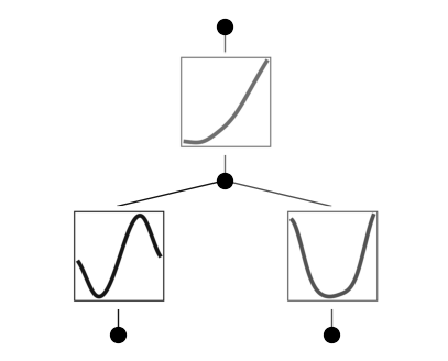

# sin appears at the top of the suggestion list, which is good!
model.suggest_symbolic(0,0,0)

function , r2
sin , 0.9981093780355159
gaussian , 0.9360582190339871
tanh , 0.8616859029524302
sigmoid , 0.8585390273680941
arctan , 0.8428622193038047

('sin',
(<function kan.utils.<lambda>(x)>, <function kan.utils.<lambda>(x)>),
0.9981093780355159)

# x^2 appears in the suggestion list (usually not top 1), but it is fine!
model.suggest_symbolic(0,1,0)

function , r2
cosh , 0.9910665391502297
x^2 , 0.9885210310683376
gaussian , 0.9883627975330689
sin , 0.9843196558672351
x^4 , 0.9403353142717915

('cosh',
(<function kan.utils.<lambda>(x)>, <function kan.utils.<lambda>(x)>),
0.9910665391502297)

# exp not even appears in the list (but note how high correlation of all these functions), which is sad!
model.suggest_symbolic(1,0,0)

function , r2
sin , 0.9995702405196035
x^2 , 0.9992413667649066
cosh , 0.9990483455142343
gaussian , 0.9989441353410312
tanh , 0.9986571504172722

('sin',
(<function kan.utils.<lambda>(x)>, <function kan.utils.<lambda>(x)>),
0.9995702405196035)

# let's try suggesting more by changing topk. Exp should appear in the list
# But it's very unclear why should we prefer exp over others. All of them have quite high correlation with the learned spline.
model.suggest_symbolic(1,0,0,topk=15)

function , r2
sin , 0.9995702405196035
x^2 , 0.9992413667649066
cosh , 0.9990483455142343
gaussian , 0.9989441353410312
tanh , 0.9986571504172722
sigmoid , 0.998657149375774
arctan , 0.9970617106973462
x^3 , 0.9962099497478061
x^4 , 0.9947572943342223
exp , 0.9913715887470934
1/x^4 , 0.9890801101893518
1/x^3 , 0.9884748093165208
1/x^2 , 0.9874565358732027
1/x , 0.9853279073610555
1/sqrt(x) , 0.9830898307444438

('sin',
(<function kan.utils.<lambda>(x)>, <function kan.utils.<lambda>(x)>),
0.9995702405196035)

让我们继续训练！损失值下降，样条曲线应该更加精确。

model.train(dataset, opt="LBFGS", steps=20);
model.plot()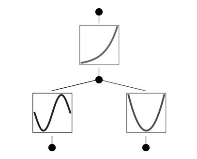

# sin appears at the top of the suggestion list, which is good!
model.suggest_symbolic(0,0,0)

function , r2
sin , 0.999987075018884
gaussian , 0.921655835107275
tanh , 0.8631397517896181
sigmoid , 0.8594117556407576
arctan , 0.8440367634049246

('sin',
(<function kan.utils.<lambda>(x)>, <function kan.utils.<lambda>(x)>),
0.999987075018884)

# x^2 appears at the top of the suggestion list, which is good!
# But note how competitive cosh and gaussian are. They are also locally quadratic.
model.suggest_symbolic(0,1,0)

function , r2
x^2 , 0.9999996930603142
cosh , 0.9999917592117541
gaussian , 0.9999827145861027
sin , 0.9980876045759569
abs , 0.9377603078924529

('x^2',
(<function kan.utils.<lambda>(x)>, <function kan.utils.<lambda>(x)>),
0.9999996930603142)

# exp appears at the top of the suggestion list, which is good!
model.suggest_symbolic(1,0,0)

function , r2
exp , 0.9999987580912774
tanh , 0.9999187437583558
cosh , 0.9999121147442106
sigmoid , 0.9998776769631791
gaussian , 0.9998535744392626

('exp',
(<function kan.utils.<lambda>(x)>, <function kan.utils.<lambda>(x)>),
0.9999987580912774)

重点在于，符号回归对噪声非常敏感，因此，如果我们想要从训练好的网络中提取精确的符号公式，网络需要达到相当高的精度！

# now let's replace every activation function with its top 1 symbolic suggestion. This is implmented in auto_symbolic()
model.auto_symbolic()

# if the user wants to constrain the symbolic space, they can pass in their symbolic libarary
# lib = ['sin', 'x^2', 'exp']
# model.auto_symbolic(lib=lib)

fixing (0,0,0) with sin, r2=0.999987075018884
fixing (0,1,0) with x^2, r2=0.9999996930603142
fixing (1,0,0) with exp, r2=0.9999987580912774

在重新训练后，我们几乎达到了机器精度！这是一个明确的信号，表明这个公式（非常有可能）是精确的！

model.train(dataset, opt="LBFGS", steps=20);
model.plot()

# obtaining symbolic formula
formula, variables = model.symbolic_formula()
formula[0]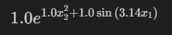

# if you want to rename your variables, you could use the "var" argument
formula, variables = model.symbolic_formula(var=['\\alpha','y'])
formula[0]

# one can even postprocess the formula (e.g., taking derivatives)
from sympy import *
diff(formula[0], variables[0])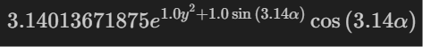

如何判断我们猜测的公式是错误的（不精确的）？如果数据是干净的（无噪声），我们应该看到训练损失没有达到机器精度

# let's replace (0,1,0) with cosh
model.fix_symbolic(0,1,0,'cosh')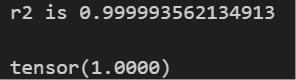

# this loss is stuck at around 1e-3 RMSE, which is good, but not machine precision.
model.train(dataset, opt="LBFGS", steps=20);
model.plot()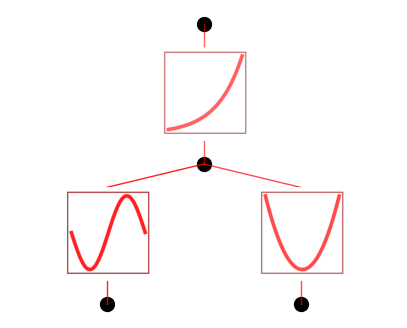

四、总结与思考

KAN神经网络通过融合数学定理与深度学习，为科学计算和可解释AI提供了新思路。尽管在高维应用中仍需突破，但其在低维复杂函数建模上的潜力值得关注。未来可能通过改进计算效率、扩展理论边界，成为MLP的重要补充。

1. KAN网络架构

关键设计：可学习的激活函数：每个网络连接的“权重”被替换为单变量函数（如样条、多项式），而非固定激活函数（如ReLU）。分层结构：输入层和隐藏层之间、隐藏层与输出层之间均通过单变量函数连接，形成多层叠加。参数效率：由于理论保证，KAN可能用更少的参数达到与MLP相当或更好的逼近效果。
示例结构：输入层 → 隐藏层：每个输入节点通过单变量函数 $\phi_{q,i} \left( x_{i} \right)$ 连接到隐藏节点。隐藏层 → 输出层：隐藏节点通过另一组单变量函数 $\psi_{q}$ 组合得到输出。