


本篇文章将会介绍在Kaggle比赛中常见的将多种模型进行集成/堆叠
参考网页:Introduction to Ensembling/Stacking in Python | Kaggle
将多个模型进行集成/堆叠的好处:
1.提高模型的泛化能力 -- 集成多个模型可以减少单个模型的过拟合,使最终的预测更加稳定和可靠
2.降低单一模型的偏差和方差 -- 单一模型通常会存在高偏差和高方差等问题,结合不同模型,可以进一步减少偏差和方差
3.结合不同模型的优点 -- 利用不同模型的优势,使最终的预测更准确
4.提高模型的鲁棒性 -- 不同模型对数据的敏感度不同,单一模型可能对某些异常值或数据分布变化过于敏感,集成多个模型可以降低这种敏感性,提高鲁棒性,使得模型更能适应数据的变化
5.降低单个模型的局限性 -- 例如:深度学习 在小样本数据上可能表现不佳,而 树模型(XGBoost、LightGBM) 可以很好地适应小样本;线性模型 可能无法很好地拟合复杂数据,而 非线性模型(SVM、神经网络) 能更好地建模。堆叠方法 结合不同模型的长处,弥补个体模型的局限性。
前期准备
在下面代码中,编写了一个类-SklearnerHelper,它允许扩展所有 Sklearn 分类器通用的内置方法(例如 train、predict 和 fit),方便后续直接调用
class SklearnHelper(object):
    # 初始化
    def __init__(self, clf, seed=0, params=None):
        params['random_state'] = seed
        self.clf = clf(**params)

    # 模型训练 -- 部分库(XGBoost、CatBoost等)的特有方法
    def train(self, x_train, y_train):
        self.clf.fit(x_train, y_train)

    # 模型训练 -- 通用训练方法(使用Sk-Learn等)
    def fit(self,x,y):
        return self.clf.fit(x,y)

    # 模型预测
    def predict(self, x):
        return self.clf.predict(x)

    # 模型训练的特征重要矩阵
    def feature_importances(self,x,y):
        print(self.clf.fit(x,y).feature_importances_)
堆叠使用基本分类器的预测作为训练到二级模型的输入,但是不能简单地在完整的训练数据上训练基础模型,在完整的测试集上生成预测,然后将这些预测输出出来用于第二级训练。这存在数据泄露的风险,因此在提供这些预测时会出现过拟合,为解决这一问题,我们需要采用交叉验证(Cross Validation, CV)的方法,来规避这一风险。
def get_oof(clf, x_train, y_train, x_test):
    '''
    clf -- 基本分类器
    x_train -- 训练集的特征
    y_train -- 训练集的标签
    x_test  -- 验证集的特征
    '''
    oof_train = np.zeros((ntrain,))
    oof_test = np.zeros((ntest,))
    oof_test_skf = np.empty((NFOLDS, ntest))

    for i, (train_index, test_index) in enumerate(kf):
        x_tr = x_train[train_index]
        y_tr = y_train[train_index]
        x_te = x_train[test_index]

        clf.train(x_tr, y_tr)

        oof_train[test_index] = clf.predict(x_te)
        oof_test_skf[i, :] = clf.predict(x_test)

    oof_test[:] = oof_test_skf.mean(axis=0)
    return oof_train.reshape(-1, 1), oof_test.reshape(-1, 1)
生成第一级基本的模型
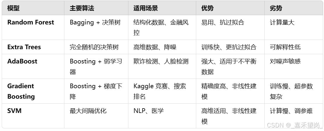
准备五个学习模型作为我们的第一级分类,以下模型可以直接通过Sk-Learn库直接调用
1.Random Forest classifier
2.Extra Trees classifier
3.AdaBoost classifer
4.Gradient Boosting classifer
5.Support Vector Machine
定义分类器的参数
# Random Forest parameters
rf_params = {
    'n_jobs': -1,
    'n_estimators': 500,
     'warm_start': True,
     #'max_features': 0.2,
    'max_depth': 6,
    'min_samples_leaf': 2,
    'max_features' : 'sqrt',
    'verbose': 0
}

# Extra Trees Parameters
et_params = {
    'n_jobs': -1,
    'n_estimators':500,
    #'max_features': 0.5,
    'max_depth': 8,
    'min_samples_leaf': 2,
    'verbose': 0
}

# AdaBoost parameters
ada_params = {
    'n_estimators': 500,
    'learning_rate' : 0.75
}

# Gradient Boosting parameters
gb_params = {
    'n_estimators': 500,
     #'max_features': 0.2,
    'max_depth': 5,
    'min_samples_leaf': 2,
    'verbose': 0
}

# Support Vector Classifier parameters
svc_params = {
    'kernel' : 'linear',
    'C' : 0.025
    }
通过SklearnHelper来创建5个对象来代表我们5个学习模型
rf = SklearnHelper(clf=RandomForestClassifier, seed=SEED, params=rf_params)
et = SklearnHelper(clf=ExtraTreesClassifier, seed=SEED, params=et_params)
ada = SklearnHelper(clf=AdaBoostClassifier, seed=SEED, params=ada_params)
gb = SklearnHelper(clf=GradientBoostingClassifier, seed=SEED, params=gb_params)
svc = SklearnHelper(clf=SVC, seed=SEED, params=svc_params)
准备输入数据(y_train、train、x_train、x_test)
y_train = train['Survived'].ravel()
train = train.drop(['Survived'], axis=1)
x_train = train.values
x_test = test.values
第一级模型输出预测输入
通过调用get_oof模型,来返回训练集的OOF预测值(适用于Stacking的第二层模型作为输入特征)和测试集的最终预测
et_oof_train, et_oof_test = get_oof(et, x_train, y_train, x_test) # Extra Trees
rf_oof_train, rf_oof_test = get_oof(rf,x_train, y_train, x_test) # Random Forest
ada_oof_train, ada_oof_test = get_oof(ada, x_train, y_train, x_test) # AdaBoost
gb_oof_train, gb_oof_test = get_oof(gb,x_train, y_train, x_test) # Gradient Boost
svc_oof_train, svc_oof_test = get_oof(svc,x_train, y_train, x_test) # Support Vector Classifier
从不同的分类器生成的特征重要性
rf_feature = rf.feature_importances(x_train,y_train)
et_feature = et.feature_importances(x_train, y_train)
ada_feature = ada.feature_importances(x_train, y_train)
gb_feature = gb.feature_importances(x_train,y_train)
'''
rf_features = [0.10474135, 0.21837029, 0.04432652, 0.02249159, 0.05432591, 0.02854371
,0.07570305, 0.01088129 , 0.24247496, 0.13685733 , 0.06128402]
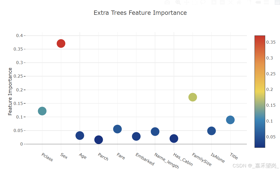
et_features = [ 0.12165657, 0.37098307 ,0.03129623 , 0.01591611 , 0.05525811 , 0.028157
,0.04589793 , 0.02030357 , 0.17289562 , 0.04853517, 0.08910063]
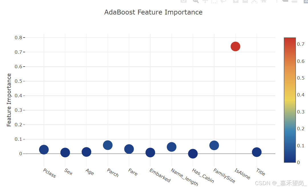
ada_features = [0.028 , 0.008 , 0.012 , 0.05866667, 0.032 , 0.008
,0.04666667 , 0. , 0.05733333, 0.73866667, 0.01066667]
gb_features = [ 0.06796144 , 0.03889349 , 0.07237845 , 0.02628645 , 0.11194395, 0.04778854
,0.05965792 , 0.02774745, 0.07462718, 0.4593142 , 0.01340093]
'''通过绘制散点图来实现交互特征重要性
# Scatter plot
trace = go.Scatter(
y = feature_dataframe['Random Forest feature importances'].values,
x = feature_dataframe['features'].values,
mode='markers',
marker=dict(
sizemode = 'diameter',
sizeref = 1,
size = 25,
# size= feature_dataframe['AdaBoost feature importances'].values,
# color = np.random.randn(500), #set color equal to a variable
color = feature_dataframe['Random Forest feature importances'].values,
colorscale='Portland',
showscale=True
),
text = feature_dataframe['features'].values
)
data = [trace]
layout= go.Layout(
autosize= True,
title= 'Random Forest Feature Importance',
hovermode= 'closest',
# xaxis= dict(
# title= 'Pop',
# ticklen= 5,
# zeroline= False,
# gridwidth= 2,
# ),
yaxis=dict(
title= 'Feature Importance',
ticklen= 5,
gridwidth= 2
),
showlegend= False
)
fig = go.Figure(data=data, layout=layout)
py.iplot(fig,filename='scatter2010')
# Scatter plot
trace = go.Scatter(
y = feature_dataframe['Extra Trees feature importances'].values,
x = feature_dataframe['features'].values,
mode='markers',
marker=dict(
sizemode = 'diameter',
sizeref = 1,
size = 25,
# size= feature_dataframe['AdaBoost feature importances'].values,
# color = np.random.randn(500), #set color equal to a variable
color = feature_dataframe['Extra Trees feature importances'].values,
colorscale='Portland',
showscale=True
),
text = feature_dataframe['features'].values
)
data = [trace]
layout= go.Layout(
autosize= True,
title= 'Extra Trees Feature Importance',
hovermode= 'closest',
# xaxis= dict(
# title= 'Pop',
# ticklen= 5,
# zeroline= False,
# gridwidth= 2,
# ),
yaxis=dict(
title= 'Feature Importance',
ticklen= 5,
gridwidth= 2
),
showlegend= False
)
fig = go.Figure(data=data, layout=layout)
py.iplot(fig,filename='scatter2010')
# Scatter plot
trace = go.Scatter(
y = feature_dataframe['AdaBoost feature importances'].values,
x = feature_dataframe['features'].values,
mode='markers',
marker=dict(
sizemode = 'diameter',
sizeref = 1,
size = 25,
# size= feature_dataframe['AdaBoost feature importances'].values,
# color = np.random.randn(500), #set color equal to a variable
color = feature_dataframe['AdaBoost feature importances'].values,
colorscale='Portland',
showscale=True
),
text = feature_dataframe['features'].values
)
data = [trace]
layout= go.Layout(
autosize= True,
title= 'AdaBoost Feature Importance',
hovermode= 'closest',
# xaxis= dict(
# title= 'Pop',
# ticklen= 5,
# zeroline= False,
# gridwidth= 2,
# ),
yaxis=dict(
title= 'Feature Importance',
ticklen= 5,
gridwidth= 2
),
showlegend= False
)
fig = go.Figure(data=data, layout=layout)
py.iplot(fig,filename='scatter2010')
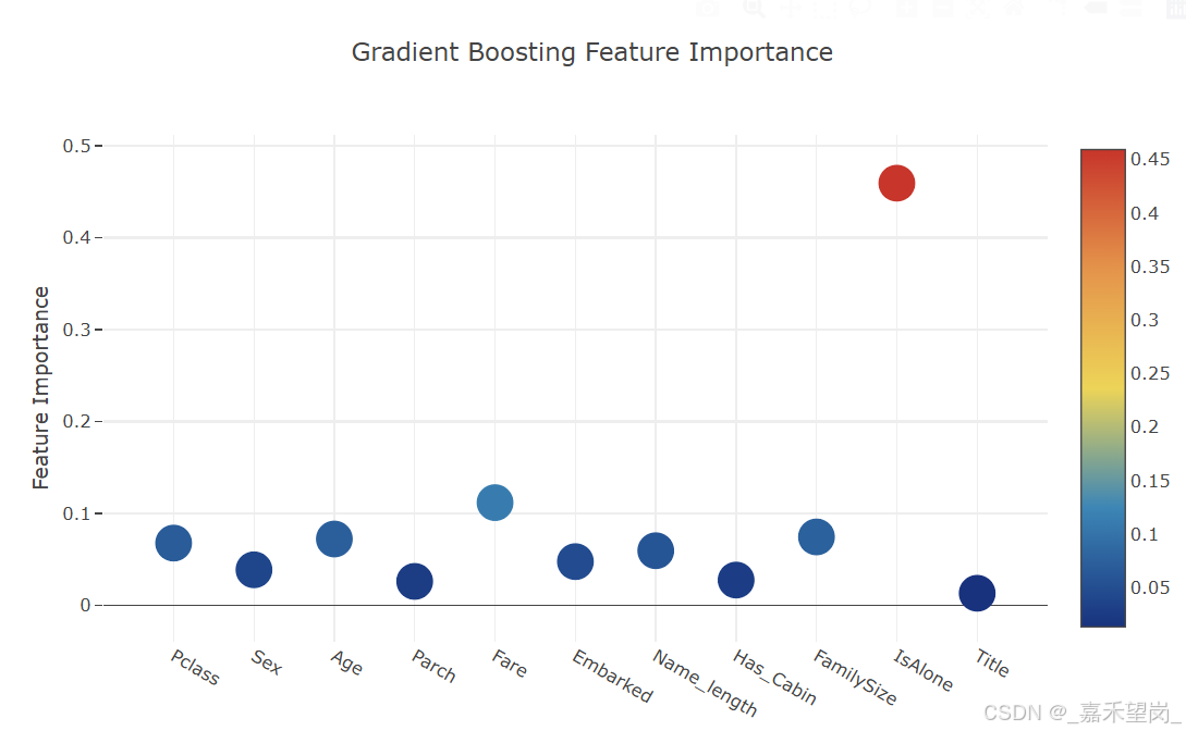
# Scatter plot
trace = go.Scatter(
y = feature_dataframe['Gradient Boost feature importances'].values,
x = feature_dataframe['features'].values,
mode='markers',
marker=dict(
sizemode = 'diameter',
sizeref = 1,
size = 25,
# size= feature_dataframe['AdaBoost feature importances'].values,
# color = np.random.randn(500), #set color equal to a variable
color = feature_dataframe['Gradient Boost feature importances'].values,
colorscale='Portland',
showscale=True
),
text = feature_dataframe['features'].values
)
data = [trace]
layout= go.Layout(
autosize= True,
title= 'Gradient Boosting Feature Importance',
hovermode= 'closest',
# xaxis= dict(
# title= 'Pop',
# ticklen= 5,
# zeroline= False,
# gridwidth= 2,
# ),
yaxis=dict(
title= 'Feature Importance',
ticklen= 5,
gridwidth= 2
),
showlegend= False
)
fig = go.Figure(data=data, layout=layout)
py.iplot(fig,filename='scatter2010')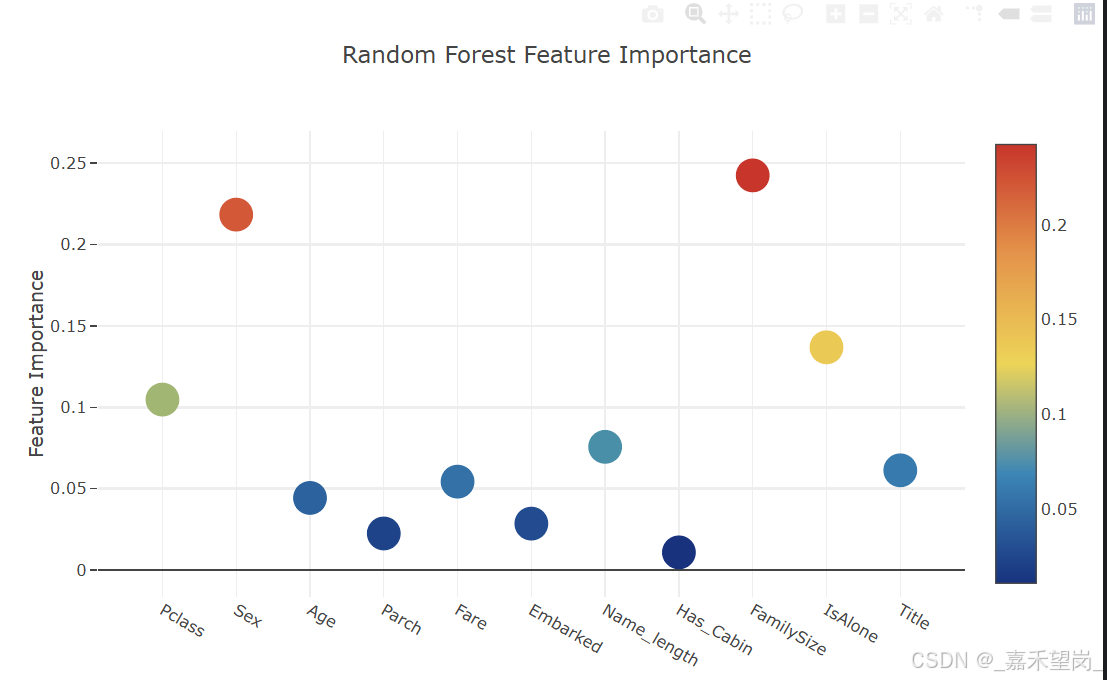
得到以上绘制的图像,现在需要计算所有特征重要性的平均值,并绘制柱状图
feature_dataframe['mean'] = feature_dataframe.mean(axis= 1)

y = feature_dataframe['mean'].values
x = feature_dataframe['features'].values
data = [go.Bar(
            x= x,
             y= y,
            width = 0.5,
            marker=dict(
               color = feature_dataframe['mean'].values,
            colorscale='Portland',
            showscale=True,
            reversescale = False
            ),
            opacity=0.6
        )]

layout= go.Layout(
    autosize= True,
    title= 'Barplots of Mean Feature Importance',
    hovermode= 'closest',
#     xaxis= dict(
#         title= 'Pop',
#         ticklen= 5,
#         zeroline= False,
#         gridwidth= 2,
#     ),
    yaxis=dict(
        title= 'Feature Importance',
        ticklen= 5,
        gridwidth= 2
    ),
    showlegend= False
)
fig = go.Figure(data=data, layout=layout)
py.iplot(fig, filename='bar-direct-labels')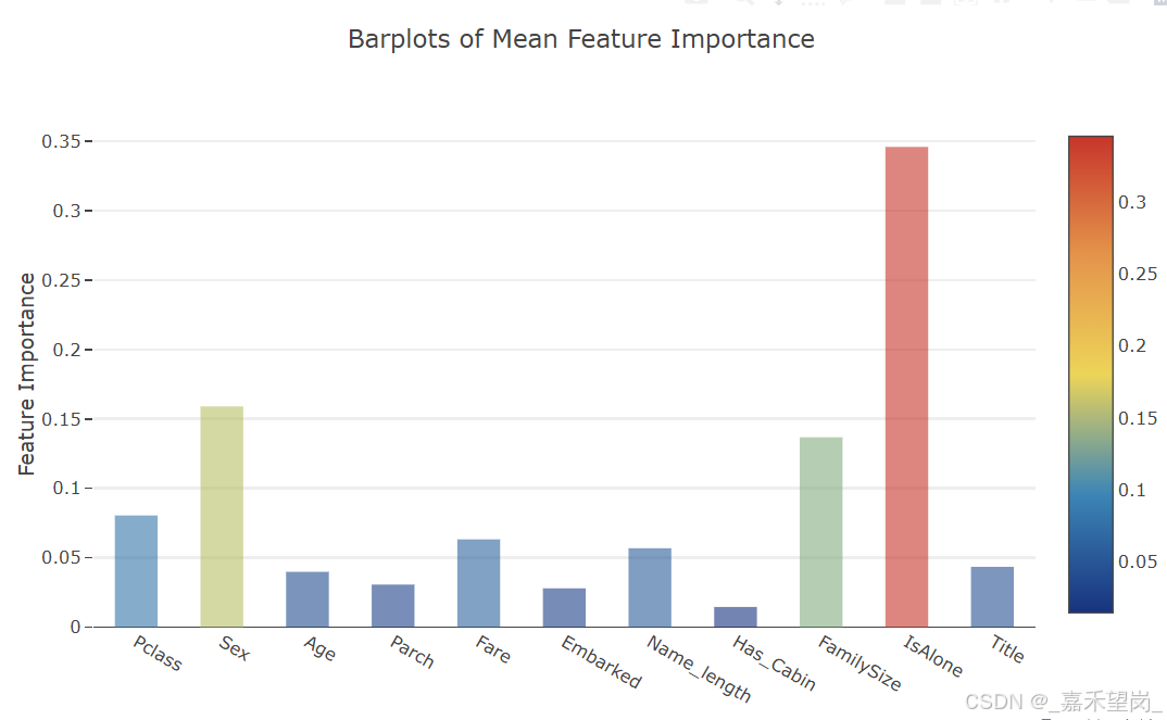
来自第一级输出的第二集预测
我们通过以上的操作,得到了第一级预测,可以将其本质视作为一组新的特征,用于下一个分类器的训练数据;因此,我们将来自早期分类器的一级预测作为我们的新列,并在此基础上训练下一个分类器
base_predictions_train = pd.DataFrame( {'RandomForest': rf_oof_train.ravel(),
     'ExtraTrees': et_oof_train.ravel(),
     'AdaBoost': ada_oof_train.ravel(),
      'GradientBoost': gb_oof_train.ravel()
    })
二级训练集的相关热力图
data = [
    go.Heatmap(
        z= base_predictions_train.astype(float).corr().values ,
        x=base_predictions_train.columns.values,
        y= base_predictions_train.columns.values,
          colorscale='Viridis',
            showscale=True,
            reversescale = True
    )
]
py.iplot(data, filename='labelled-heatmap')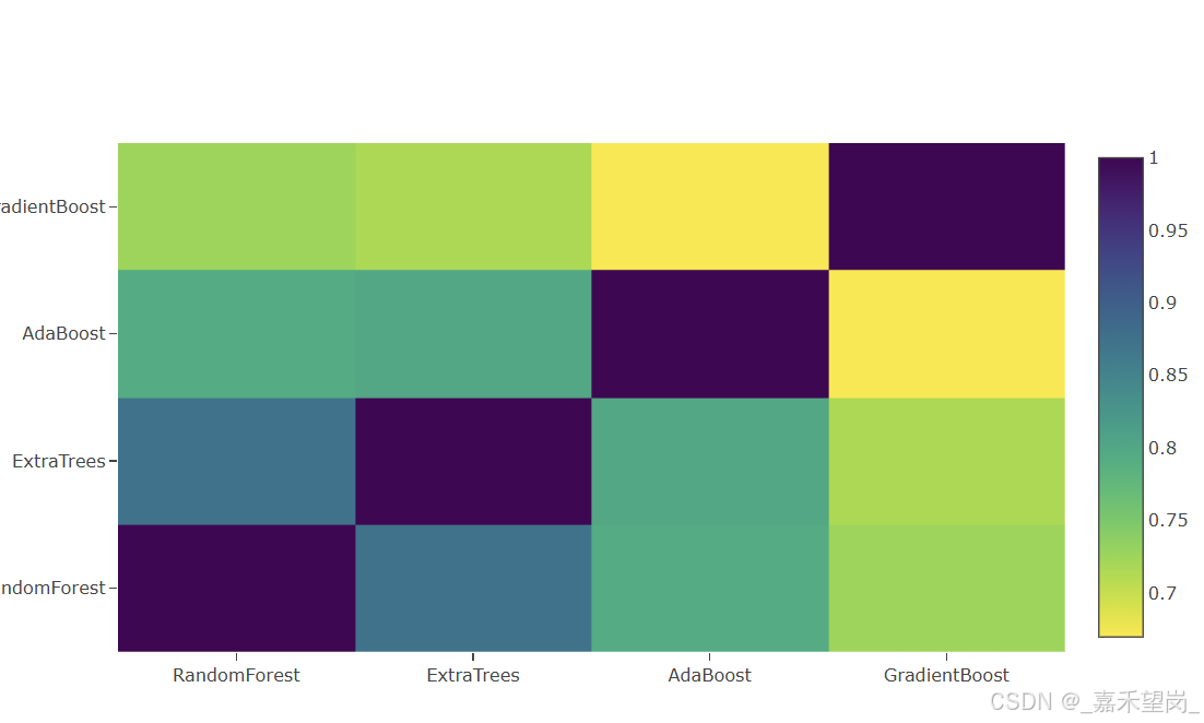
现在,我们将第一级训练和测试集预测连接为x_train和x_test,我们将拟合第二级学习模型
x_train = np.concatenate(( et_oof_train, rf_oof_train, ada_oof_train, gb_oof_train, svc_oof_train), axis=1)
x_test = np.concatenate(( et_oof_test, rf_oof_test, ada_oof_test, gb_oof_test, svc_oof_test), axis=1)
通过XGBoost的第二级学习模型
我们调用 XGBClassifier 并将其拟合到一级训练和目标数据,并使用学习到的模型来预测测试数据
gbm = xgb.XGBClassifier(
    #learning_rate = 0.02,
 n_estimators= 2000,
 max_depth= 4,
 min_child_weight= 2,
 #gamma=1,
 gamma=0.9,
 subsample=0.8,
 colsample_bytree=0.8,
 objective= 'binary:logistic',
 nthread= -1,
 scale_pos_weight=1).fit(x_train, y_train)
predictions = gbm.predict(x_test)
进一步的改进:
1.在训练模型时实施良好的交叉验证策略以找到最佳参数值
2.引入更多种类的学习基础模型,结果越不相关,最终分数越高


 1万+
1万+

 被折叠的 条评论
为什么被折叠?
被折叠的 条评论
为什么被折叠?
 到【灌水乐园】发言


