


C++第十九讲:Hash使用和Hash实现
1.Hash系列概念阐述
1.1什么是哈希
哈希又称散列,有散乱排列的意思,它既不是顺序表那样顺序排列,又不是二叉树那样树状排列,而是散乱排列
哈希的本质是通过哈希函数将key和存储位置之间建立映射关系,在查找时再通过哈希函数计算出key值存储的位置,进行快速查找
1.2哈希冲突
映射方法有很多种,例如直接定址法,在存储关键字连续的情况下十分好用,比如26个英文字母的存储,我们只需开辟26个空间大小,通过英文字母的ASCII码进行映射即可,但是这对于散乱的关键字映射有很大的局限性,使用直接定址法会浪费很多不用的空间,所以我们要采取一个方法,使这个方法能够开辟固定空间(例如100)的存储数组,能够将key值为1和key值为1000的数据都能够通过哈希函数映射到存储数组中
但是正常情况下还会遇到哈希冲突的问题,也就是两个key值通过哈希函数映射到了同一块存储空间中,所以对于哈希冲突我们也要尽量进行避免,因为哈希冲突实质上是不可避免的,还要实现解决策略
1.3负载因子
假设哈希表中已经映射存储了N个值,哈希表的大小是M,那么负载因子等于N/M,负载因子太大,会导致每次映射都有很大可能会造成哈希冲突,而负载因子太小,会导致空间利用率太低,所以一般会将负载因子控制在小于0.7,当负载因子等于0.7时,会进行扩容操作
2.哈希函数
哈希函数其实就是映射关系的实现,一个好的哈希函数要能够尽量减少哈希冲突,也就是将N个关键字被等概率地散布到哈希表的M个空间中
2.1除法散列法/除留余数法(下面将要实现)
1.除法散列法也叫作除留余数法,也就是key/M,保留余数,这样就可以将不管多大的数据控制在小于M的范围内,此时的哈希函数为:h(key) = key % M
2.当使用除法散列法时,应该避免M为某些值,如2的幂,10的幂。如果是2的幂,那么key%2^x,本质是保留key二进制位中的后x位,也就是说当key的二进制表示中,后x位相同的元素映射的位置相同。如63(111111)和31(11111),%16的值都是15(1111)
3.通过大佬的研究发现,M建议取不太接近2的次数幂的一个质数(素数)
4.但是方法并不唯一,Java实现的HashMap中,哈希函数为取2的次数幂,比如对于一个32位的数来说,取2的16次幂,本质是保留后16位的数据,但是实现时取出前16位的数据和后16位的数据进行了异或,实现了减少哈希冲突的目的
2.2乘法散列法(了解)
1.乘法散列法的优点是对于M没有要求,它的大致思路为:使用关键字key乘上一个小数A(0<A<1),抽出KA的小数部分,然后使用M乘上小数部分,向下取整得出映射位置
2.此时的哈希函数为:h(key) = floor(M(key*A)%1.0),floor表示对表达式进行向下取整,A属于0-1,Knuth认为,A = (根号5 - 1)/2,也就是黄金分割点比较好
2.3全域散列法(了解)
1.全域散列法适用于针对特殊情况的一种方法,当别人恶意破解映射函数时,可能会插入一系列的会造成哈希冲突的数据集,让所有的数据都通过映射函数映射到同一处位置,这会使得我们的代码效率低下
2.该方法的哈希函数为:h(key) = ((a*key + b) % P) % M,a的取值范围为[1, p-1],b的取值范围为[0, p-1],这使得每一次的哈希函数都不同,就很难被恶意攻击破解了
3.这里需要注意的是,初始化哈希表之后,需要固定哈希函数,也就是随机值的取值需要固定,防止后序找不到映射关系
当然还有其它的方法,如平方取中法、折叠法、随机数法等,感兴趣的话自己查找
3.处理哈希冲突
哈希冲突无法避免,所以我们要找到方法尽量避免哈希冲突的发生,而且还要有哈希冲突发生时的解决方法
3.1开放定址法
开放定址法中,所有元素都存储在哈希表中,是一一对应的关系,当发生哈希冲突是,按照规则插入到没有存储数据的位置上,这里的规则有三种:线性探测、二次探测、双重探测
3.1.1线性探测
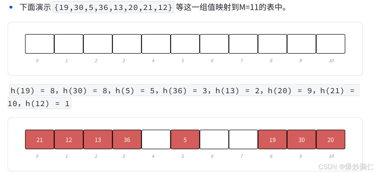
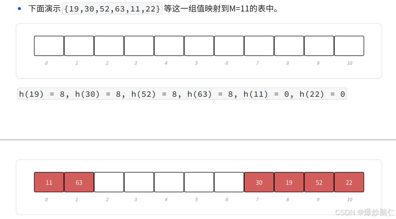
1.线性探测的大概思路为:从发生冲突的位置开始,向后依次查询,直到查找到一个没有存储数据的位置即可,如果走到哈希表尽头,那么从头部开始进行查找
2.探测公式为:h(key) = hash0 = key % M;
hc(key, i) = hashi = (hash0+i) % M,i = {1,2,3,M-1}
3.当hash0,hash1,hash2都映射在同一个位置时,hash1和hash2会向后进行移动,那么后续如果有数据映射到了hash1和hash2的位置时,就会发生连锁反应,造成后续的哈希冲突,下面的二次映射可以一定程度上改善这类问题
3.1.2二次探测
1.该方法并不是像线性探测那样,在冲突的位置向后依次进行查找,而是向后跳跃式查找
2.探测公式为:h(key) = hash0 = key % M;
hc(key, i) = hashi = (hash0 ± i^2) % M, i = {1, 2, 3, ……M/2};
3.当hash0 <= 0时,需要hashi += M
3.1.3双重散列(了解)
1.该方法的思路为:使用第一个哈希函数进行映射,出现哈希冲突时,使用第二个哈希函数计算偏移量,不断向后探测,直到查找到一个没有存储数据的位置为止
2.公式为:h1(key) = hash0 = key % M,hash0位置冲突了,双重探测公式为:hc(key, i) = (hash0 + i*h2(key)) % M,i = {1, 2, 3, ……M}
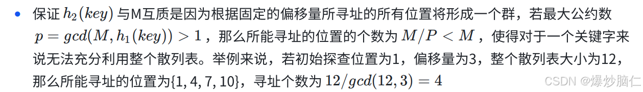
3.这里要求h2(key) < M而且h2(key)和M互为质数,有两种简单的取值方法:1.M为2的次数幂时,h2(key)从[0, M-1]任选一个奇数 2.M为质数时,h2(key) = key % (M-1) + 1
3.2开放定址法代码实现
这里我们使用线性探测法和除留余数法进行代码实现
3.2.1哈希表框架
enum State
{
	EXIST,
	EMPTY,
	DELETE
};

template<class K, class V>
class HashData
{
	pair<K, V> _kv;
	State _state = EMPTY;
};

template<class K, class V>
class HashTable
{
public:


private:
	vector<pair<K, V>> _tables;
};
3.2.2Insert函数实现
class HashTable
{
public:
	HashTable()
	{
		_tables.resize(__stl_next_prime(1));//初始开辟53的空间大小
	}

	//扩容数据,返回大于n的最小扩容数
	inline unsigned long __stl_next_prime(unsigned long n)
	{
		//Note: assumes long is at least 32 bits.
		static const int __stl_num_primes = 28;
		static const unsigned long __stl_prime_list[__stl_num_primes] =
		{
			53, 97, 193, 389, 769,
			1543, 3079, 6151, 12289, 24593,
			49157, 98317, 196613, 393241, 786433,
			1572869, 3145739, 6291469, 12582917, 25165843,
			50331653, 100663319, 201326611, 402653189, 805306457,
			1610612741, 3221225473, 4294967291
		};
		const unsigned long* first = __stl_prime_list;
		const unsigned long* last = __stl_prime_list + __stl_num_primes;
		const unsigned long* pos = lower_bound(first, last, n);
		return pos == last ? *(last - 1) : *pos;
	}

	bool Insert(const pair<K, V>& kv)
	{
		//当负载因子大于0.7时,需要进行扩容
		if ((double)_n / (double)_tables.size() >= 0.7)
		{
			//上面说过,线性映射对M的大小有要求,所以扩容的大小有要求

			方法一,创建一个新的哈希表,但是需要重新更新数据
			//size_t newSize = __stl_next_prime(_tables.size()+1);
			//vector<pair<K, V>> newtables(newSize);
			//for (int i = 0; i < _tables.size(); i++)
			//{
			//	//进行数据转移操作
			//}
			//_tables.swap(newtables);

			//方法二:直接创建一个新的哈希表,将原来哈希表中的数据遍历重新插入到该哈希表中
			size_t newSize = __stl_next_prime(_tables.size() + 1);
			HashTable<K, V> newHT;
			newHT._tables.resize(newSize);
			for (int i = 0; i < _tables.size(); i++)
			{
				newHT.Insert(_tables[i]._kv);//使用函数调用,省略自己写的步骤
			}
			_tables.swap(newHT._tables);
		}

		//1.找到映射位置
		int M = _tables.size();
		size_t hash0 = kv.first % M;
		size_t hashi = hash0;
		size_t i = 1;
		while (_tables[hashi]._state == EXIST)
		{
			//2.当映射位置存在时,需要使用线性探测解决哈希冲突
			hashi = (hash0 + i) % M;
			i++;
		}
		_tables[hashi]._kv = kv;
		_tables[hashi]._state = EXIST;
		_n++;
	}

private:
	vector<HashData<K, V>> _tables;
	size_t _n = 0;//表中存储的数据的个数
};
3.2.3Find函数 && Erase函数实现
HashData<K, V>* Find(const K& key)
{
	size_t hash0 = key % _tables.size();
	size_t hashi = hash0;
	size_t i = 0;
	while (_tables[hashi]._state != EMPTY)
	{
		if (_tables[hashi]._kv.first == key &&
			_tables[hashi]._state == EXIST)
		{
			return &_tables[hashi];
		}
		hashi = (hash0 + i) % _tables.size();
		i++;
	}
	return nullptr;
}

bool Erase(const K& key)
{
	HashData<K, V>* ret = Find(key);
	if (ret == nullptr)
	{
		return false;
	}
	else
	{
		--_n;
		ret->_state = DELETE;
		return true;
	}
}
3.2.5插入代码优化
在插入代码中,我们使用hash0 = key % M来进行映射,但是对于字符串来说,并没有key值,所以我们要针对于字符串类型做出特殊处理,这里我们采用字符串的所有字符的ASCII码相加进行处理,但是对于abc和cba,映射出的结果是一样的,所以我们还有进行乘法处理:
template<class K>
class HashFunc
{
public:
	size_t operator()(const K& key)
	{
		return (size_t)key;
	}
};

//模板特化
template<>
class HashFunc<string>
{
public:
	size_t operator()(const string& key)
	{
		size_t hash = 0;
		for (auto ch : key)
		{
			hash += ch;
			hash *= 131;
		}
		return hash;
	}
};

/*class StringHashFunc
{
public:
	size_t operator()(const string& key)
	{
		size_t hash = 0;
		for (auto ch : key)
		{
			hash += ch;
			hash *= 131;
		}
		return hash;
	}
};*/

void TestHT2()
{
	//HashTable<string, string, StringHashFunc> ht2;
	HashTable<string, string> ht2;
	ht2.Insert({ "sort", "排序" });
	ht2.Insert({ "string", "字符串" });
}
3.2.4全部代码实现
namespace YWL
{
enum State
{
EXIST,
EMPTY,
DELETE
};
template<class K, class V>
struct HashData
{
pair<K, V> _kv;
State _state = EMPTY;
};
template<class K>
class HashFunc
{
public:
size_t operator()(const K& key)
{
return (size_t)key;
}
};
//模板特化
template<>
class HashFunc<string>
{
public:
size_t operator()(const string& key)
{
size_t hash = 0;
for (auto ch : key)
{
hash += ch;
hash *= 131;
}
return hash;
}
};
/*class StringHashFunc
{
public:
size_t operator()(const string& key)
{
size_t hash = 0;
for (auto ch : key)
{
hash += ch;
hash *= 131;
}
return hash;
}
};*/
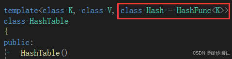
template<class K, class V, class Hash = HashFunc<K>>
class HashTable
{
public:
HashTable()
{
_tables.resize(__stl_next_prime(1));//初始开辟53的空间大小
}
//扩容数据,返回大于n的最小扩容数
inline unsigned long __stl_next_prime(unsigned long n)
{
//Note: assumes long is at least 32 bits.
static const int __stl_num_primes = 28;
static const unsigned long __stl_prime_list[__stl_num_primes] =
{
53, 97, 193, 389, 769,
1543, 3079, 6151, 12289, 24593,
49157, 98317, 196613, 393241, 786433,
1572869, 3145739, 6291469, 12582917, 25165843,
50331653, 100663319, 201326611, 402653189, 805306457,
1610612741, 3221225473, 4294967291
};
const unsigned long* first = __stl_prime_list;
const unsigned long* last = __stl_prime_list + __stl_num_primes;
const unsigned long* pos = lower_bound(first, last, n);
return pos == last ? *(last - 1) : *pos;
}
bool Insert(const pair<K, V>& kv)
{
if (Find(kv.first)) return false;//不允许重复的key值插入
//当负载因子大于0.7时,需要进行扩容
if ((double)_n / (double)_tables.size() >= 0.7)
{
//上面说过,线性映射对M的大小有要求,所以扩容的大小有要求
方法一,创建一个新的哈希表,但是需要重新更新数据
//size_t newSize = __stl_next_prime(_tables.size()+1);
//vector<pair<K, V>> newtables(newSize);
//for (int i = 0; i < _tables.size(); i++)
//{
// //进行数据转移操作
//}
//_tables.swap(newtables);
//方法二:直接创建一个新的哈希表,将原来哈希表中的数据遍历重新插入到该哈希表中
size_t newSize = __stl_next_prime(_tables.size() + 1);
HashTable<K, V, Hash> newHT;
newHT._tables.resize(newSize);
for (int i = 0; i < _tables.size(); i++)
{
newHT.Insert(_tables[i]._kv);//使用函数调用,省略自己写的步骤
}
_tables.swap(newHT._tables);
}
//1.找到映射位置
int M = _tables.size();
Hash hs;
size_t hash0 = hs(kv.first) % M;
size_t hashi = hash0;
size_t i = 1;
while (_tables[hashi]._state == EXIST)
{
//2.当映射位置存在时,需要使用线性探测解决哈希冲突
hashi = (hash0 + i) % M;
i++;
}
_tables[hashi]._kv = kv;
_tables[hashi]._state = EXIST;
_n++;
}
HashData<K, V>* Find(const K& key)
{
Hash hs;
size_t hash0 = hs(key) % _tables.size();
size_t hashi = hash0;
size_t i = 0;
while (_tables[hashi]._state != EMPTY)
{
if (_tables[hashi]._kv.first == key &&
_tables[hashi]._state == EXIST)
{
return &_tables[hashi];
}
hashi = (hash0 + i) % _tables.size();
i++;
}
return nullptr;
}
bool Erase(const K& key)
{
HashData<K, V>* ret = Find(key);
if (ret == nullptr)
{
return false;
}
else
{
--_n;
ret->_state = DELETE;
return true;
}
}
private:
vector<HashData<K, V>> _tables;
size_t _n = 0;//表中存储的数据的个数
};
void TestHT1()
{
HashTable<int, int> ht1;
ht1.Insert({ 54, 1 });
ht1.Insert({ 1, 1 });
cout << ht1.Find(1) << endl;
cout << ht1.Erase(54) << endl;
cout << ht1.Find(1) << endl;
cout << ht1.Find(54) << endl;
for (int i = 0; i < 53; i++)
{
ht1.Insert({rand(), i});
}
}
void TestHT2()
{
//HashTable<string, string, StringHashFunc> ht2;
HashTable<string, string> ht2;
ht2.Insert({ "sort", "排序" });
ht2.Insert({ "string", "字符串" });
}
}
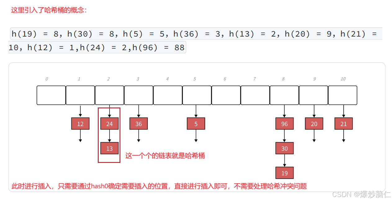
3.3链地址法
3.3.1链地址法的实现思路
开放定址法实现的哈希表,需要通过hash0定位哈希表的位置,再通过hashi处理哈希冲突,而在链地址法实现的哈希表中,并不需要使用hashi来处理哈希冲突:
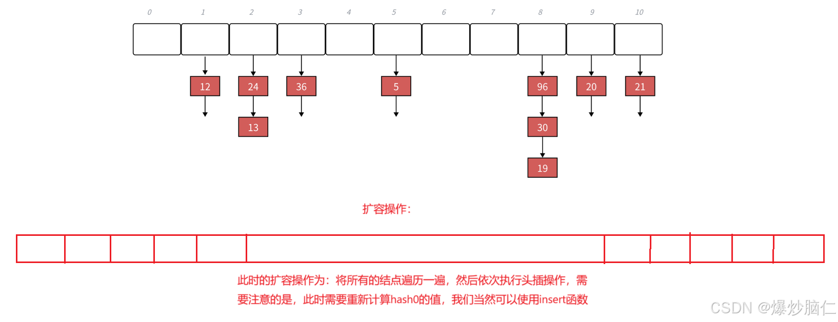
3.3.2Insert函数实现
inline unsigned long __stl_next_prime(unsigned long n)
{
	static const int __stl_num_primes = 28;
	static const unsigned long __stl_prime_list[__stl_num_primes] =
	{
		53, 97, 193, 389, 769,
		1543, 3079, 6151, 12289, 24593,
		49157, 98317, 196613, 393241, 786433,
		1572869, 3145739, 6291469, 12582917, 25165843,
		50331653, 100663319, 201326611, 402653189, 805306457,
		1610612741, 3221225473, 4294967291
	};
	const unsigned long* first = __stl_prime_list;
	const unsigned long* last = __stl_prime_list + __stl_num_primes;
	const unsigned long* pos = lower_bound(first, last, n);
	return pos == last ? *(last - 1) : *pos;
}

bool Insert(cosnt pair<K, V>& kv)
{
	//当负载因子等于1时,进行扩容操作
	if (_n == _table.size())
	{
		size_t newcapacity = __stl_next_prime(_tables.size()+1);
		vector<Node*> newTables(newcapacity, nullptr);
		for (int i = 0; i < _tables.size(); i++)
		{
			Node* cur = _tables[i];
			while (cur)
			{
				Node* next = cur->next;
				size_t hash0 = cur->_kv.first % newcapacity;
				cur->next = newTables[i];
				newTables[i] = cur;

				cur = next;
			}
			_tables[i] = nullptr;//这点需要注意,需要将原表置空
		}
		_tables.swap(newTables);
	}

	size_t hash0 = kv.first % _tables.size();
	Node* newnode = new Node(kv);
	//直接头插到哈希桶中
	newnode->next = _table[hash0];
	_tables[hash0] = newnode;
	_n++;
}
3.3.3Find函数实现
Node* Find(const K& key)
{
	size_t hash0 = key % _tables.size();
	Node* cur = _tables[hash0];
	while (cur)
	{
		if (cur->_kv.first == key)
		{
			return cur;
		}
		cur = cur->next;
	}
	return nullptr;
}
3.3.4析构函数的实现
因为该方法实现的哈希表是vector<Node*>类型的,因为vector有自己的析构函数,但是Node*没有自己的析构函数,所以如果不自定义析构函数的话,编译器只会将vector数组进行析构,并不会将哈希桶里面的结点进行析构
vector<Node*> _tables;
~HashTable()
{
	//依次把每个桶析构
	for (int i = 0; i < _tables.size(); i++)
	{
		Node* cur = _tables[i];
		while (cur)
		{
			Node* next = cur->next;
			delete cur;
			cur = next;
		}
		_tables[i] = nullptr;
	}
}
3.3.5删除函数的实现
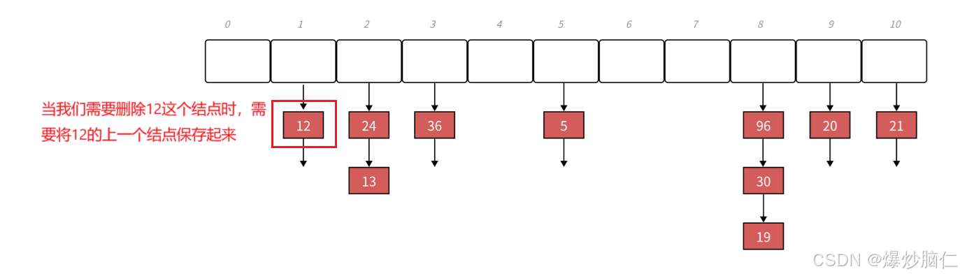
bool Erase(const K& key)
{
	size_t hash0 = key % _tables.size();
	Node* pcur = nullptr;
	Node* cur = _tables[hash0];
	while (cur)
	{
		if (cur->_kv.first == key)
		{
			if (pcur == nullptr)
			{
				_tables[hash0] = cur->next;
			}
			else
			{
				pcur->next = cur->next;
			}
			delete cur;
			return true;
		}
		pcur = cur;
		cur = cur->next;
	}
	return false;
}
3.4链地址法代码实现
//哈希桶的哈希实现
namespace hash_bucket
{
	template<class K, class V>
	struct HashNode
	{
		pair<K, V> _kv;
		HashNode* next;

		HashNode(const pair<K, V>& kv)
			:_kv(kv)
			,next(nullptr)
		{}
	};

	template<class K, class V>
	class HashTable
	{
		typedef HashNode<K, V> Node;
	public:
		HashTable()
		{
			_tables.resize(__stl_next_prime(1), nullptr);
		}

		~HashTable()
		{
			//依次把每个桶析构
			for (int i = 0; i < _tables.size(); i++)
			{
				Node* cur = _tables[i];
				while (cur)
				{
					Node* next = cur->next;
					delete cur;
					cur = next;
				}
				_tables[i] = nullptr;
			}
		}

		inline unsigned long __stl_next_prime(unsigned long n)
		{
			static const int __stl_num_primes = 28;
			static const unsigned long __stl_prime_list[__stl_num_primes] =
			{
				53, 97, 193, 389, 769,
				1543, 3079, 6151, 12289, 24593,
				49157, 98317, 196613, 393241, 786433,
				1572869, 3145739, 6291469, 12582917, 25165843,
				50331653, 100663319, 201326611, 402653189, 805306457,
				1610612741, 3221225473, 4294967291
			};
			const unsigned long* first = __stl_prime_list;
			const unsigned long* last = __stl_prime_list + __stl_num_primes;
			const unsigned long* pos = lower_bound(first, last, n);
			return pos == last ? *(last - 1) : *pos;
		}

		bool Insert(const pair<K, V>& kv)
		{
			if (Find(kv.first)) return false;

			//当负载因子等于1时,进行扩容操作
			if (_n == _tables.size())
			{
				size_t newcapacity = __stl_next_prime(_tables.size()+1);
				vector<Node*> newTables(newcapacity, nullptr);
				for (int i = 0; i < _tables.size(); i++)
				{
					Node* cur = _tables[i];
					while (cur)
					{
						Node* next = cur->next;
						size_t hash0 = cur->_kv.first % newcapacity;
						cur->next = newTables[i];
						newTables[i] = cur;

						cur = next;
					}
					_tables[i] = nullptr;//这点需要注意,需要将原表置空
				}
				_tables.swap(newTables);
			}

			size_t hash0 = kv.first % _tables.size();
			Node* newnode = new Node(kv);
			//直接头插到哈希桶中
			newnode->next = _tables[hash0];
			_tables[hash0] = newnode;
			_n++;
		}

		Node* Find(const K& key)
		{
			size_t hash0 = key % _tables.size();
			Node* cur = _tables[hash0];
			while (cur)
			{
				if (cur->_kv.first == key)
				{
					return cur;
				}
				cur = cur->next;
			}
			return nullptr;
		}

		bool Erase(const K& key)
		{
			size_t hash0 = key % _tables.size();
			Node* pcur = nullptr;
			Node* cur = _tables[hash0];
			while (cur)
			{
				if (cur->_kv.first == key)
				{
					if (pcur == nullptr)
					{
						_tables[hash0] = cur->next;
					}
					else
					{
						pcur->next = cur->next;
					}
					delete cur;
					return true;
				}
				pcur = cur;
				cur = cur->next;
			}
			return false;
		}

	private:
		vector<Node*> _tables;
		size_t _n = 0;
	};

	void TestHT1()
	{
		HashTable<int, int> ht1;
		ht1.Insert({ 54, 1 });
		ht1.Insert({ 1, 1 });

		for (int i = 0; i < 53; i++)
		{
			ht1.Insert({ rand(), i });
		}

		ht1.Erase(19895);
		ht1.Erase(15724);
	}
}


 被折叠的 条评论
为什么被折叠?
被折叠的 条评论
为什么被折叠?
 到【灌水乐园】发言


