


前言
本文并非正式的变种LSTM模型介绍,只是把一些比较火的技术,像双向注意力机制,自注意力机制这样的比较火的内容,简单的和LSTM堆叠,结果发现效果都不如最基础的,这里作者将本人代码及实现结果,进行展示,给各位想更改LSTM的朋友一些借鉴/教训。
使用数据集
C-MAPSS(Commercial Modular Aero-Propulsion System Simulation)数据集是由 NASA 发布的一个用于涡扇发动机剩余寿命预测(RUL, Remaining Useful Life)的数据集。它是航空发动机故障预测和健康管理(PHM, Prognostics and Health Management)领域的标准测试数据集,广泛用于 数据驱动的预测性维护 研究。
关于数据集一个很好的介绍:C-MAPSS数据集详细介绍_cmapss数据集-优快云博客
数据集下载:N-CMAPSS数据集下载链接-优快云博客
这个数据解释不太好,还没有header,直接看比较难理解,如果事先没接触过这个数据集的朋友,最后详细阅读以下readme文件和上面推荐的介绍链接。
数据预处理
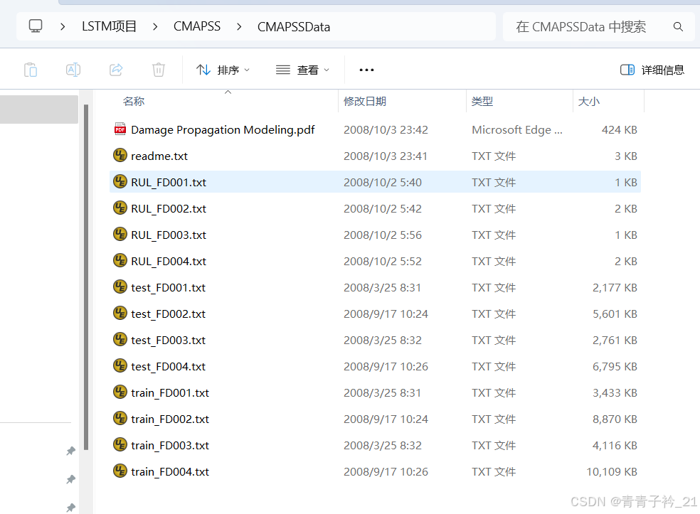
数据集一共有四份文件(不是四个),针对一组train,test,rul分别有FD001-FD004四个文件,如下所示:
首先导入必要的库
import pandas as pd
import numpy as np
import matplotlib.pyplot as plt
import torch
import torch.nn as nn
import torch.optim as optim
from sklearn.metrics import mean_squared_error下面我提供两份读取文件的代码,分别是读取单份数据的(简单快速),以及处理整体数据的(总体但较慢),两份代码任选一份即可。
## 1.1 加载数据

# 数据格式
# 数据以 文本文件 形式存储,每行表示某台发动机在某个周期的状态,共 26 个列:

# unit number(发动机编号)
# time, in cycles(当前运行周期)
# 3-5. operational setting 1-3(操作设置参数,影响发动机性能)
# 6-26. sensor measurement 1-26(26 个传感器数据,监测发动机状态)

# 使用正则表达式 '\s+' 作为分隔符,避免多余空格导致的错误列
train_df = pd.read_csv('CMAPSS_Data/train_FD001.txt', sep=r'\s+', header=None, engine='python')
test_df = pd.read_csv('CMAPSS_Data/test_FD001.txt', sep=r'\s+', header=None, engine='python')
rul_df = pd.read_csv('CMAPSS_Data/RUL_FD001.txt', sep=r'\s+', header=None, engine='python')

# 重新命名列
columns = ['unit', 'time', 'op1', 'op2', 'op3'] + [f'sensor_{i}' for i in range(1, 22)]
train_df.columns = columns
test_df.columns = columns

train_df.head()  # 检查数据
## 1.1 加载数据

# 数据格式
# 数据以 文本文件 形式存储,每行表示某台发动机在某个周期的状态,共 26 个列:

# unit number(发动机编号)
# time, in cycles(当前运行周期)
# 3-5. operational setting 1-3(操作设置参数,影响发动机性能)
# 6-26. sensor measurement 1-26(26 个传感器数据,监测发动机状态)

# 使用正则表达式 '\s+' 作为分隔符,避免多余空格导致的错误列
import pandas as pd

# 数据文件列表
train_files = ['CMAPSS_Data/train_FD001.txt', 'CMAPSS_Data/train_FD002.txt',
               'CMAPSS_Data/train_FD003.txt', 'CMAPSS_Data/train_FD004.txt']

test_files = ['CMAPSS_Data/test_FD001.txt', 'CMAPSS_Data/test_FD002.txt',
              'CMAPSS_Data/test_FD003.txt', 'CMAPSS_Data/test_FD004.txt']

rul_files = ['CMAPSS_Data/RUL_FD001.txt', 'CMAPSS_Data/RUL_FD002.txt',
             'CMAPSS_Data/RUL_FD003.txt', 'CMAPSS_Data/RUL_FD004.txt']

# 读取并拼接训练数据
train_df_list = [pd.read_csv(f, sep=r'\s+', header=None, engine='python') for f in train_files]
train_df = pd.concat(train_df_list, ignore_index=True)

# 读取并拼接测试数据
test_df_list = [pd.read_csv(f, sep=r'\s+', header=None, engine='python') for f in test_files]
test_df = pd.concat(test_df_list, ignore_index=True)

# 读取并拼接 RUL 数据
rul_df_list = [pd.read_csv(f, sep=r'\s+', header=None, engine='python') for f in rul_files]
rul_df = pd.concat(rul_df_list, ignore_index=True)

# 重新命名列名
columns = ['unit', 'time', 'op1', 'op2', 'op3'] + [f'sensor_{i}' for i in range(1, 22)]
train_df.columns = columns
test_df.columns = columns

print(train_df.shape, test_df.shape, rul_df.shape)  # 查看拼接后的数据维度
train_df.head()  # 查看拼接后的数据
然后是数据预处理,转换成标准形式,把真实的答案,也就是RUL合并到最后一列,下面分别是训练集和测试集的处理。
## 1.2 计算训练集的 RUL

# 计算最大循环数(最大时间步)并反向计算 RUL
max_cycles = train_df.groupby('unit')['time'].max()
train_df = train_df.merge(max_cycles.to_frame(name='max_time'), on='unit')
train_df['RUL'] = train_df['max_time'] - train_df['time']
train_df.drop(columns=['max_time'], inplace=True)
train_df
## 1.3 测试集导入真实 RUL
# 计算测试集 RUL
max_cycles_test = test_df.groupby('unit')['time'].max().reset_index()
max_cycles_test.columns = ['unit', 'max_time']
# rul_df 是按 unit 顺序存储的,给它加上 unit 索引
rul_df['unit'] = max_cycles_test['unit']
rul_df.columns = ['rul_max', 'unit']
# 合并测试数据与 RUL
test_df = test_df.merge(max_cycles_test, on='unit')
test_df = test_df.merge(rul_df, on='unit')
# 计算真实 RUL
test_df['RUL'] = (test_df['max_time'] - test_df['time']) + test_df['rul_max']
test_df.drop(columns=['max_time', 'rul_max'], inplace=True)
test_df.head()归一化处理,为了加速lstm计算
from sklearn.preprocessing import MinMaxScaler

# 选择需要归一化的列(去掉 ID 和时间步)
feature_cols = train_df.columns.difference(['unit', 'time', 'RUL'])

scaler = MinMaxScaler()
train_df[feature_cols] = scaler.fit_transform(train_df[feature_cols])
test_df[feature_cols] = scaler.transform(test_df[feature_cols])
生成lstm需要的时间步数据,也就是说,数据是三维的,分别表示特征、时间步、数据量(也就是把原先的数据量-特征的二维数据,给拉伸成三维的,从而方便之后更好的代入长短期时间序列这一模型)。
sequence_length = 50

def create_sequences(df, sequence_length):
    """ 生成 LSTM 所需的时间序列数据 """
    sequences = []
    labels = []

    for unit in df['unit'].unique():
        unit_df = df[df['unit'] == unit].sort_values(by='time')
        features = unit_df[feature_cols].values
        target = unit_df['RUL'].values

        for i in range(len(unit_df) - sequence_length):
            sequences.append(features[i:i+sequence_length])
            labels.append(target[i+sequence_length])

    return np.array(sequences), np.array(labels)

X_train, y_train = create_sequences(train_df, sequence_length)
X_test, y_test = create_sequences(test_df, sequence_length)

X_train
array([[[1.90400484e-04, 2.37360551e-04, 1.00000000e+00, ...,
9.62152586e-01, 9.98776165e-01, 8.42549679e-01],
[9.99926220e-01, 9.97626394e-01, 1.00000000e+00, ...,
2.73789803e-03, 6.26983457e-01, 2.59356549e-01],
[1.95160496e-04, 1.18680275e-03, 1.00000000e+00, ...,
9.61255292e-01, 9.98565159e-01, 8.55231414e-01],
...,
[2.42760617e-04, 1.89888441e-03, 1.00000000e+00, ...,
9.61163262e-01, 9.98902768e-01, 8.36716716e-01],
[4.76215410e-01, 8.31474009e-01, 1.00000000e+00, ...,
4.58218296e-01, 8.63331364e-01, 5.76058663e-01],
[5.95175252e-01, 7.36529789e-01, 0.00000000e+00, ...,
8.82569483e-02, 1.18163403e-03, 1.23484223e-02]],基础LSTM
## 模型训练 ##

class LSTMRUL(nn.Module):
    def __init__(self, input_size, hidden_size, num_layers):
        super(LSTMRUL, self).__init__()
        self.lstm = nn.LSTM(input_size, hidden_size, num_layers, batch_first=True)
        self.fc = nn.Linear(hidden_size, 1)  # 回归任务,输出一个值

    def forward(self, x):
        lstm_out, _ = self.lstm(x)
        out = self.fc(lstm_out[:, -1, :])  # 取最后一个时间步的输出
        return out

# 超参数
input_size = X_train.shape[2]  # 传感器数量
hidden_size = 64
num_layers = 2
lr = 0.0015
epochs = 60
batch_size = 64

# 初始化模型
model = LSTMRUL(input_size, hidden_size, num_layers)
criterion = nn.MSELoss()
optimizer = optim.Adam(model.parameters(), lr=lr)

from torch.utils.data import DataLoader, TensorDataset

# 转换为 PyTorch Tensor
X_train_tensor = torch.tensor(X_train, dtype=torch.float32)
y_train_tensor = torch.tensor(y_train, dtype=torch.float32).unsqueeze(1)
X_test_tensor = torch.tensor(X_test, dtype=torch.float32)
y_test_tensor = torch.tensor(y_test, dtype=torch.float32).unsqueeze(1)

train_dataset = TensorDataset(X_train_tensor, y_train_tensor)
train_loader = DataLoader(train_dataset, batch_size=batch_size, shuffle=True)

# 训练循环
device = torch.device("cuda" if torch.cuda.is_available() else "cpu")
model.to(device)

# 记录损失
first_loss_history = []

for epoch in range(epochs):
    model.train()
    total_loss = 0

    for batch_X, batch_y in train_loader:
        batch_X, batch_y = batch_X.to(device), batch_y.to(device)

        optimizer.zero_grad()
        output = model(batch_X)
        loss = criterion(output, batch_y)
        loss.backward()
        optimizer.step()

        total_loss += loss.item()

    avg_loss = total_loss / len(train_loader)  # 计算平均损失
    first_loss_history.append(avg_loss)  # 记录损失

    print(f'Epoch {epoch+1}/{epochs}, Loss: {total_loss/len(train_loader)}')

print("训练完成!")
## 模型评估 ##

model.eval()
with torch.no_grad():
    predictions_baselstm = model(X_test_tensor.to(device)).cpu().numpy()

# 计算 RMSE 误差
from sklearn.metrics import mean_squared_error

rmse = np.sqrt(mean_squared_error(y_test, predictions_baselstm))
print(f'测试 RMSE: {rmse}')
## 结果分析 ##

import matplotlib.pyplot as plt

plt.figure(figsize=(10, 5))
plt.plot(y_test[:], label="True RUL", linestyle='dashed')
plt.plot(predictions_baselstm[:], label="Predicted RUL")
plt.legend()
plt.xlabel("Sample")
plt.ylabel("RUL")
plt.title("RUL Prediction using LSTM")
plt.show()
双向注意力 + LSTM
## 模型训练 ##

import torch
import torch.nn as nn
import torch.optim as optim

class Attention(nn.Module):
    def __init__(self, hidden_size):
        super(Attention, self).__init__()
        self.attn = nn.Linear(hidden_size * 2, 1)  # 计算注意力权重
        self.softmax = nn.Softmax(dim=1)  # 归一化

    def forward(self, lstm_out):
        attn_weights = self.softmax(self.attn(lstm_out))  # 计算注意力权重
        attn_applied = torch.sum(attn_weights * lstm_out, dim=1)  # 加权求和
        return attn_applied

class BiLSTMAttention(nn.Module):
    def __init__(self, input_size, hidden_size, num_layers):
        super(BiLSTMAttention, self).__init__()
        self.lstm = nn.LSTM(input_size, hidden_size, num_layers, batch_first=True, bidirectional=True)
        self.attention = Attention(hidden_size)
        self.fc = nn.Linear(hidden_size * 2, 1)  # 最终输出 RUL 值

    def forward(self, x):
        lstm_out, _ = self.lstm(x)  # 双向 LSTM 输出
        attn_out = self.attention(lstm_out)  # 应用注意力
        out = self.fc(attn_out)  # 通过全连接层输出
        return out

# 超参数
input_size = X_train.shape[2]  # 传感器特征数
hidden_size = 64
num_layers = 2
lr = 0.0015
epochs = 60
batch_size = 64

# 初始化模型
model = BiLSTMAttention(input_size, hidden_size, num_layers)
criterion = nn.MSELoss()
optimizer = optim.Adam(model.parameters(), lr=lr)

# 训练循环
device = torch.device("cuda" if torch.cuda.is_available() else "cpu")
model.to(device)

from torch.utils.data import DataLoader, TensorDataset

X_train_tensor = torch.tensor(X_train, dtype=torch.float32)
y_train_tensor = torch.tensor(y_train, dtype=torch.float32).unsqueeze(1)
train_dataset = TensorDataset(X_train_tensor, y_train_tensor)
train_loader = DataLoader(train_dataset, batch_size=batch_size, shuffle=True)

# 记录损失
second_loss_history = []

for epoch in range(epochs):
    model.train()
    total_loss = 0

    for batch_X, batch_y in train_loader:
        batch_X, batch_y = batch_X.to(device), batch_y.to(device)

        optimizer.zero_grad()
        output = model(batch_X)
        loss = criterion(output, batch_y)
        loss.backward()
        optimizer.step()

        total_loss += loss.item()

    avg_loss = total_loss / len(train_loader)  # 计算平均损失
    second_loss_history.append(avg_loss)  # 记录损失

    print(f'Epoch {epoch+1}/{epochs}, Loss: {total_loss/len(train_loader)}')

print("训练完成!")
## 模型评估 ##

model.eval()
with torch.no_grad():
    predictions_bilstm = model(torch.tensor(X_test, dtype=torch.float32).to(device)).cpu().numpy()

from sklearn.metrics import mean_squared_error
rmse = np.sqrt(mean_squared_error(y_test, predictions_bilstm))
print(f'测试 RMSE: {rmse}')
## 结果展示 ##
import matplotlib.pyplot as plt
plt.figure(figsize=(10, 5))
plt.plot(y_test[:], label="True RUL", linestyle='dashed')
plt.plot(predictions_bilstm[:], label="Predicted RUL")
plt.legend()
plt.xlabel("Sample")
plt.ylabel("RUL")
plt.title("RUL Prediction using LSTM")
plt.show()
双向注意力 + 自注意力机制 + LSTM
## 模型训练 ##

import torch
import torch.nn as nn
import torch.optim as optim

class SelfAttention(nn.Module):
    def __init__(self, hidden_size):
        super(SelfAttention, self).__init__()
        self.query = nn.Linear(hidden_size * 2, hidden_size * 2)  # 双向 LSTM 输出的大小是 hidden_size*2
        self.key = nn.Linear(hidden_size * 2, hidden_size * 2)
        self.value = nn.Linear(hidden_size * 2, hidden_size * 2)
        self.softmax = nn.Softmax(dim=1)

    def forward(self, lstm_out):
        # 计算 Q、K、V
        query = self.query(lstm_out)
        key = self.key(lstm_out)
        value = self.value(lstm_out)

        # 计算 attention 权重
        attention_scores = torch.bmm(query, key.transpose(1, 2))  # 点积 Q 和 K
        attention_weights = self.softmax(attention_scores)  # Softmax 计算权重

        # 得到加权的 V
        attn_out = torch.bmm(attention_weights, value)
        return attn_out, attention_weights

class BiLSTMSelfAttention(nn.Module):
    def __init__(self, input_size, hidden_size, num_layers):
        super(BiLSTMSelfAttention, self).__init__()
        self.lstm = nn.LSTM(input_size, hidden_size, num_layers, batch_first=True, bidirectional=True)
        self.attention = SelfAttention(hidden_size)
        self.fc = nn.Linear(hidden_size * 2, 1)  # 输出 RUL 值

    def forward(self, x):
        lstm_out, _ = self.lstm(x)  # 双向 LSTM 输出
        attn_out, attention_weights = self.attention(lstm_out)  # 自注意力加权
        attn_out = torch.sum(attn_out, dim=1)  # 按时间步维度加权求和
        out = self.fc(attn_out)  # 通过全连接层输出 RUL
        return out, attention_weights

# 超参数
input_size = X_train.shape[2]  # 传感器特征数
hidden_size = 64
num_layers = 2
lr = 0.0015
epochs = 60
batch_size = 64

# 初始化模型
model = BiLSTMSelfAttention(input_size, hidden_size, num_layers)
criterion = nn.MSELoss()
optimizer = optim.Adam(model.parameters(), lr=lr)

# 训练循环
device = torch.device("cuda" if torch.cuda.is_available() else "cpu")
model.to(device)

from torch.utils.data import DataLoader, TensorDataset

X_train_tensor = torch.tensor(X_train, dtype=torch.float32)
y_train_tensor = torch.tensor(y_train, dtype=torch.float32).unsqueeze(1)
train_dataset = TensorDataset(X_train_tensor, y_train_tensor)
train_loader = DataLoader(train_dataset, batch_size=batch_size, shuffle=True)

# 记录损失
third_loss_history = []

for epoch in range(epochs):
    model.train()
    total_loss = 0

    for batch_X, batch_y in train_loader:
        batch_X, batch_y = batch_X.to(device), batch_y.to(device)

        optimizer.zero_grad()
        output, _ = model(batch_X)
        loss = criterion(output, batch_y)
        loss.backward()
        optimizer.step()

        total_loss += loss.item()

    avg_loss = total_loss / len(train_loader)  # 计算平均损失
    third_loss_history.append(avg_loss)  # 记录损失

    print(f'Epoch {epoch+1}/{epochs}, Loss: {total_loss/len(train_loader)}')

print("训练完成!")
## 模型评估 ##

# 评估
model.eval()
with torch.no_grad():
    predictions_selfattention, attention_weights = model(torch.tensor(X_test, dtype=torch.float32).to(device))

from sklearn.metrics import mean_squared_error
rmse = np.sqrt(mean_squared_error(y_test, predictions_selfattention.cpu().numpy()))
print(f'测试 RMSE: {rmse}')
## 可视化注意力权重 ##
import matplotlib.pyplot as plt
plt.figure(figsize=(10, 5))
plt.plot(attention_weights.cpu().numpy().flatten(), label="Attention Weights", linestyle='dashed')
plt.legend()
plt.xlabel("Time Step")
plt.ylabel("Attention Weight")
plt.title("Attention Weights Visualization")
plt.show()## 结果展示 ##
import matplotlib.pyplot as plt
plt.figure(figsize=(10, 5))
plt.plot(y_test[:], label="True RUL", linestyle='dashed')
plt.plot(predictions_selfattention.cpu()[:], label="Predicted RUL")
plt.legend()
plt.xlabel("Sample")
plt.ylabel("RUL")
plt.title("RUL Prediction using LSTM")
plt.show()
双向注意力 + 自注意力机制 + LSTM + 改进损失函数
改进损失函数将 MSE (均方误差) 改为 Huber Loss(胡泊损失),均方误差对异常值(Outliers)非常敏感,因为误差平方后放大了大误差的影响,可能导致模型过度拟合异常值;Huber Loss 结合了 MSE 和 MAE(平均绝对误差) 的优点,能够减小异常值的影响,提高模型的鲁棒性。
| 比较项 | MSE(均方误差) | Huber Loss(胡泊损失) |
|---|---|---|
| 数学形式 | 误差的平方 | 结合 MSE 和 MAE |
| 对小误差 | 计算平方,梯度平滑 | 计算平方,梯度平滑 |
| 对大误差(异常值) | 放大影响,易受异常值影响 | 采用 MAE,减少异常值影响 |
| 鲁棒性 | 较差,异常值影响大 | 较强,对异常值不敏感 |
| 收敛速度 | 慢,因异常值影响梯度 | 快,因减少异常值影响 |
| 适用场景 | 无异常值的回归任务 | 存在异常值的回归任务 |
## 模型训练 ##

import torch
import torch.nn as nn
import torch.optim as optim
import numpy as np

class BiLSTMAttention(nn.Module):
    def __init__(self, input_size, hidden_size, num_layers):
        super(BiLSTMAttention, self).__init__()

        self.bilstm = nn.LSTM(input_size, hidden_size, num_layers,
                              batch_first=True, bidirectional=True)

        # 注意力层
        self.attention = nn.Linear(hidden_size * 2, 1)  # 双向LSTM输出维度为 hidden_size * 2
        self.softmax = nn.Softmax(dim=1)

        # 全连接层用于回归预测
        self.fc = nn.Linear(hidden_size * 2, 1)

    def forward(self, x):
        lstm_out, _ = self.bilstm(x)  # BiLSTM 输出 (batch, seq_len, hidden_size*2)

        # 计算注意力权重
        attention_weights = self.attention(lstm_out)  # (batch, seq_len, 1)
        attention_weights = self.softmax(attention_weights)  # 归一化

        # 加权求和,得到最终的上下文向量
        context_vector = torch.sum(attention_weights * lstm_out, dim=1)  # (batch, hidden_size*2)

        # 通过全连接层预测 RUL
        out = self.fc(context_vector)  # (batch, 1)
        return out

# **自定义改进损失函数**
# Huber Loss(胡泊损失) 替代————> MSELoss(均方误差)
class HuberLoss(nn.Module):
    """ Huber Loss (Smooth L1 Loss) """
    def __init__(self, delta=1.0):
        super(HuberLoss, self).__init__()
        self.delta = delta

    def forward(self, y_pred, y_true):
        error = y_true - y_pred
        is_small_error = torch.abs(error) <= self.delta
        squared_loss = 0.5 * error ** 2
        linear_loss = self.delta * (torch.abs(error) - 0.5 * self.delta)
        return torch.mean(torch.where(is_small_error, squared_loss, linear_loss))

# 超参数
input_size = X_train.shape[2]  # 传感器数量
hidden_size = 64
num_layers = 2
lr = 0.0015
epochs = 60
batch_size = 64

# 初始化模型
model = BiLSTMAttention(input_size, hidden_size, num_layers)
criterion = HuberLoss(delta=1.0)  # 使用 Huber 损失
optimizer = optim.Adam(model.parameters(), lr=lr)

# 训练数据转换为 PyTorch Tensor
X_train_tensor = torch.tensor(X_train, dtype=torch.float32)
y_train_tensor = torch.tensor(y_train, dtype=torch.float32).unsqueeze(1)
X_test_tensor = torch.tensor(X_test, dtype=torch.float32)
y_test_tensor = torch.tensor(y_test, dtype=torch.float32).unsqueeze(1)

from torch.utils.data import DataLoader, TensorDataset

train_dataset = TensorDataset(X_train_tensor, y_train_tensor)
train_loader = DataLoader(train_dataset, batch_size=batch_size, shuffle=True)

# 训练循环
device = torch.device("cuda" if torch.cuda.is_available() else "cpu")
model.to(device)

# 记录损失
fourth_loss_history = []

for epoch in range(epochs):
    model.train()
    total_loss = 0

    for batch_X, batch_y in train_loader:
        batch_X, batch_y = batch_X.to(device), batch_y.to(device)

        optimizer.zero_grad()
        output = model(batch_X)
        loss = criterion(output, batch_y)
        loss.backward()
        optimizer.step()

        total_loss += loss.item()

    avg_loss = total_loss / len(train_loader)  # 计算平均损失
    fourth_loss_history.append(avg_loss)  # 记录损失
    print(f'Epoch {epoch+1}/{epochs}, Loss: {total_loss/len(train_loader)}')

print("训练完成!")
## 模型评估 ##

model.eval()
with torch.no_grad():
    predictions_loss = model(X_test_tensor.to(device)).cpu().numpy()

# 计算 RMSE
rmse = np.sqrt(mean_squared_error(y_test, predictions_loss))
print(f'测试 RMSE: {rmse}')
## 结果展示 ##
# 绘图
plt.figure(figsize=(10, 5))
plt.plot(y_test[:], label="True RUL", linestyle='dashed')
plt.plot(predictions_loss[:], label="Predicted RUL") # 这里不需要 .cpu()
plt.legend()
plt.xlabel("Sample")
plt.ylabel("RUL")
plt.title("RUL Prediction using BiLSTM + Attention")
plt.show()损失函数可视化
import matplotlib.pyplot as plt

# 创建主图
fig, ax1 = plt.subplots(figsize=(8, 5))

# 主 Y 轴
ax1.plot(range(1, epochs+1), first_loss_history, marker='.', linestyle='-', label="lstm")
ax1.plot(range(1, epochs+1), second_loss_history, marker='.', linestyle='-', label="bilstm")
ax1.plot(range(1, epochs+1), third_loss_history, marker='.', linestyle='-', label="bilstm + self-attention")

# 创建次 Y 轴
ax2 = ax1.twinx()
ax2.plot(range(1, epochs+1), fourth_loss_history, marker='x', linestyle='-', color='red', label="lstm with another loss")

# 轴标签
ax1.set_xlabel('Epochs')
ax1.set_ylabel('MSE Loss')
ax2.set_ylabel('Huber Loss')

# 设置图例
ax1.legend(loc='upper right', bbox_to_anchor=(1, 1))
ax2.legend(loc='upper right', bbox_to_anchor=(1, 0.80))  # 往下移

# 标题 & 网格
plt.title('Training Loss Curve')
plt.grid(True)

# 显示图像
plt.show()
下面展示的是单个数据集FD001的损失函数,可以看出,因为数据的逻辑结构过于简单,因此最后都收敛了,基础LSTM在前期收敛较慢。
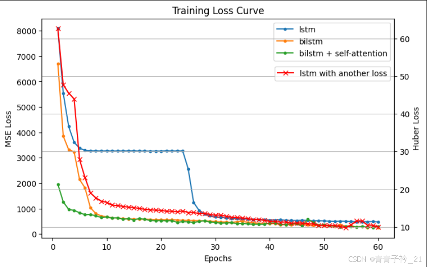
但是基础lstm的MSE是最低的,可见并不是越复杂的模型效果一定越好,越复杂的模型可能效果更差,如下所示,越复杂均方误差越大。
| lstm | 33.9612795943933 |
| bilstm | 38.667340147295754 |
| bilstm+self-attention | 35.95792461237371 |
| bilstm+self-attention + loss | 40.4522131330351 |


 被折叠的 条评论
为什么被折叠?
被折叠的 条评论
为什么被折叠?
 到【灌水乐园】发言


