基于一阶梯度算子的边缘检测方法——Roberts 算子、Prewitt 算子、Sobel 算子

涵涵不是憨憨~

已于 2024-08-25 14:46:57 修改

阅读量1.3k

点赞数 8

分类专栏： # 图像处理文章标签： python 图像处理

于 2024-08-24 20:13:05 首次发布

本文链接：https://blog.youkuaiyun.com/2201_75691823/article/details/141503360

版权

图像处理专栏收录该内容

6 篇文章

订阅专栏

文章目录

基础知识
一、基于梯度算子的检测算法
- 1.1 基于一阶梯度算子的方法

基础知识

边缘：一般指图象中像素强度局部剧烈变化的区域。

边缘检测的目标：找到图像中像素强度局部剧烈变化的像素点的集合。

一、基于梯度算子的检测算法

梯度本意是一个向量（矢量），表示某一函数在该点处的方向导数沿着该方向取得最大值，即函数在该点处沿着该方向（此梯度的方向）变化最快，变化率最大（该梯度的模）。

1.1 基于一阶梯度算子的方法

设在图象 $(x, y)$ 处，像素值为 $f (x, y)$ 。则该处水平与垂直方向的梯度为：

$\left\{\begin{matrix} \frac{\partial f(x,y)}{\partial x} = \lim_{\varepsilon \to 0\frac{f(x+\varepsilon ,y)-f(x,y)}{\varepsilon }} \\ \frac{\partial f(x,y)}{\partial y} = \lim_{\varepsilon \to 0\frac{f(x ,y+\varepsilon)-f(x,y)}{\varepsilon }} \end{matrix}\right.$

因为图像的坐标是离散的，在图像中1是最接近0的变化量。所以 $\varepsilon = 1$ ，进而可得：

$\left\{\begin{matrix} \frac{\partial f(x,y)}{\partial x} = f(x+1,y)-f(x,y) \\ \frac{\partial f(x,y)}{\partial y} = f(x,y+1)-f(x,y) \end{matrix}\right.$

所以，梯度的模（值）为：

$\sqrt{({\frac{\partial f(x,y)}{\partial x})^2} + {(\frac{\partial f(x,y)}{\partial y})^2}}$

1.1.1 Roberts 算子

（1）原理

当不沿 x 轴和 y 轴计算梯度，而是沿着 45 度和 -45度求梯度时，梯度值为
$G(x,y)=\sqrt{(f(x+1,y+1)-f(x,y))^{2}+(f(x,y+1)-f(x+1,y)^{2})}$

有时为了进一步简化计算，可按如下近似公式计算。
$G (x, y) = ∣ f (x + 1, y + 1) - f (x, y) ∣ + ∣ f (x, y + 1) - f (x + 1, y) ∣$
【注：沿着x轴和y轴时，最小的像素间隔是 1 像素；沿着 45 度和 -45度时最小的像素间隔应该是 $\sqrt{2}$ ，为什么没有体现。答：我也不清楚，可能是整体乘除不改变大小关系，所以为了简化计算分母还用的1？】

之后我们再看 Roberts 算子的两个2×2 的卷积核，
$G(x)=\begin{bmatrix}1&0\\0&-1\end{bmatrix}$

$G(y)=\begin{bmatrix}{0}&{1}\\{-1}&{0}\end{bmatrix}$

可以发现其分别对应 -45度直线和 45度直线的梯度计算。

所以用 Roberts 算子进行边缘检测时，需要使用上述两个卷积核，对图像进行卷积，然后计算梯度值，并根据自定义的阈值大小，判断该像素点是否为边缘即可。

（2）代码

可以先简单了解一下边缘检测会用到的函数，详见 opencv-python 4 函数笔记。

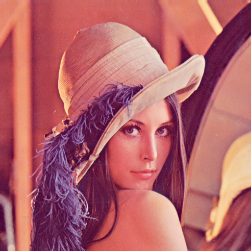
在测试阶段使用经典图像：
请添加图片描述

首先定义些公共数据
BASE_DATA.py

"""
边缘检测的一些公共路径和参数
date：2024/7/28
"""

IMAGE_PATH = r'D:\优快云\ImageProcessing\EdgeDetection\source\Lena.jpg'  # 图片输入路径
RESULT_DIR = r'D:\优快云\ImageProcessing\EdgeDetection\result'  # 图片输出文件夹
THRESHOLD = 50  # 梯度阈值

之后调用 filter2D 实现 Roberts 算子。
Roberts_operator.py

"""
Roberts operator
date：2024/8/2
"""
import cv2
import numpy as np
import BASE_DATA

# 定义Roberts算子的卷积核
kernel_x = np.array([[1, 0], [0, -1]])
kernel_y = np.array([[0, 1], [-1, 0]])

def Roberts_operator(image_path=BASE_DATA.IMAGE_PATH, threshold=BASE_DATA.THRESHOLD):
    image = cv2.imread(image_path, cv2.IMREAD_GRAYSCALE)
    image_16 = image.astype(np.int16)
    # 计算梯度
    gradient_x = cv2.filter2D(image_16, -1, kernel_x)
    gradient_y = cv2.filter2D(image_16, -1, kernel_y)

    gradient_magnitude = np.clip(np.abs(gradient_x) + np.abs(gradient_y), 0, 255).astype(np.uint8)  # 梯度近似取值

    # 将高于阈值的像素设为白色
    edges = np.zeros_like(gradient_magnitude)  # 生成大小与 gradient_magnitude 一致的全 0 数组
    edges[gradient_magnitude > threshold] = 255

    # 显示结果
    cv2.imshow('Original grayscale image', image)
    cv2.imshow('Gradient image', gradient_magnitude)
    cv2.imshow('Edge image', edges)

    cv2.waitKey(0)
    cv2.destroyAllWindows()

    return edges

if __name__ == '__main__':
    image_path = BASE_DATA.IMAGE_PATH
    edges = Roberts_operator(image_path, BASE_DATA.THRESHOLD)
    # 保存边缘检测结果到文件
    out_path = BASE_DATA.RESULT_DIR + r'\Roberts.png'
    cv2.imwrite(out_path, edges)

当然也可以编写卷积函数实现。
Roberts_operator_bottom.py

"""
稍微底层一些的 Roberts operator
主要实现了卷积操作
date：2024/8/2
"""
import cv2
import numpy as np
import BASE_DATA

# convolution
def convolve(image, kernel):
    kernel_height, kernel_width = kernel.shape
    height, width = image.shape
    padded_image = np.zeros((height + 1, width + 1), dtype=np.int32)
    for i in range(0, height + 1):
        for j in range(0, width + 1):
            if i == 0 and j == 0:
                padded_image[0, 0] = image[1, 1]
                continue
            elif i == 0 and j >= 1:
                padded_image[0, j] = image[1, j - 1]
            elif j == 0 and i >= 1:
                padded_image[i, 0] = image[i - 1, 1]
            else:
                padded_image[i, j] = image[i - 1, j - 1]
    result = np.zeros((height, width), dtype=np.int32)

    for i in range(1, height + 1):
        for j in range(1, width + 1):
            result[i - 1, j - 1] = (kernel[0, 0] * padded_image[i - 1, j - 1]
                                    + kernel[1, 0] * padded_image[i, j - 1]
                                    + kernel[0, 1] * padded_image[i - 1, j]
                                    + kernel[1, 1] * padded_image[i, j]
                                    )

    return result

kernel_x = np.array([[1, 0], [0, -1]])
kernel_y = np.array([[0, 1], [-1, 0]])

def Roberts_operator_bottom(image_path=BASE_DATA.IMAGE_PATH, threshold=BASE_DATA.THRESHOLD):
    image = cv2.imread(image_path, cv2.IMREAD_GRAYSCALE)
    image_16 = image.astype(np.int16)

    gradient_x = convolve(image_16, kernel_x)
    gradient_y = convolve(image_16, kernel_y)

    gradient_magnitude = np.clip(np.abs(gradient_x) + np.abs(gradient_y), 0, 255).astype(np.uint8)

    edges = np.zeros_like(gradient_magnitude)
    edges[gradient_magnitude > threshold] = 255

    cv2.imshow('Original grayscale image', image)
    cv2.imshow('Gradient image', gradient_magnitude)
    cv2.imshow('Edge image', edges)

    cv2.waitKey(0)
    cv2.destroyAllWindows()

    return edges

if __name__ == '__main__':
    image_path = BASE_DATA.IMAGE_PATH
    edges = Roberts_operator_bottom(image_path, BASE_DATA.THRESHOLD)
    out_path = BASE_DATA.RESULT_DIR + r'\Roberts.png'
    cv2.imwrite(out_path, edges)

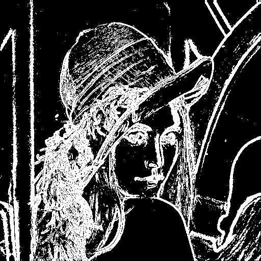
（3）结果

运行上述 Roberts_operator.py 或 Roberts_operator_bottom.py 可以得到：

原图像的灰度图
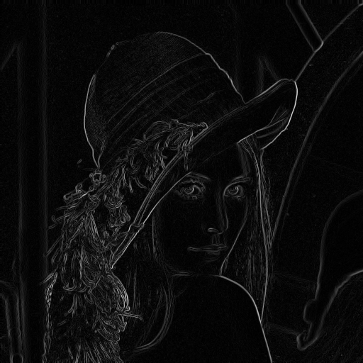
灰度图的 Roberts 算子梯度图
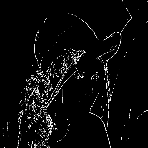
灰度图的 Roberts 算子的二值图、边缘图

可以测试下两种实现方法结果是否一样。
test_Roberts_equal.py

import numpy as np
import Roberts_operator
import Roberts_operator_bottom

edge1 = Roberts_operator.Roberts_operator()
edge2 = Roberts_operator_bottom.Roberts_operator_bottom()

if np.array_equal(edge1, edge2):
    print("Arrays are equal.")
else:
    print("Arrays are not equal.")

最后输出为 Arrays are equal. 说明两种实现方式得到的结果是否相同， Roberts 算子边缘检测程序实现完毕。

（4）优缺点

简单快速：Roberts算子只使用2x2的小型滤波器，计算量较小，实现起来非常简单快捷。

1.1.2 Prewitt 算子

（1）原理

与 Roberts 算子相似，Prewitt 算子由两个 3x3 矩阵构成，一个用于检测水平边缘（Gx），另一个用于检测垂直边缘（Gy）。

$G_x = \begin{bmatrix} -1 & 0 & 1 \\ -1 & 0 & 1 \\ -1 & 0 & 1 \\ \end{bmatrix}$

$G_y = \begin{bmatrix} 1 & 1 & 1 \\ 0 & 0 & 0 \\ -1 & -1 & -1 \\ \end{bmatrix}$

以 Gx 为例，将其作用于原图像 (x,y) 处时，可得到 $G_x = f(x+1,y+1)-f(x-1,y+1) + f(x+1,y)-f(x-1,y)+f(x+1,y-1)-f(x-1,y-1)$

（2）代码

具体实现时与 Roberts 算子流程一致。

Prewitt_operator.py

"""
Prewitt operator
date：2024/8/2
"""
import cv2
import numpy as np
import BASE_DATA

# 定义Prewitt算子的卷积核
kernel_x = np.array([[-1, 0, 1],
                     [-1, 0, 1],
                     [-1, 0, 1]])
kernel_y = np.array([[1, 1, 1],
                     [0, 0, 0],
                     [-1, -1, -1]])

def Prewitt_operator(image_path=BASE_DATA.IMAGE_PATH, threshold=BASE_DATA.THRESHOLD):
    # 读取灰度图像
    image = cv2.imread(image_path, cv2.IMREAD_GRAYSCALE)
    image_16 = image.astype(np.int16)

    # 计算梯度
    gradient_x = cv2.filter2D(image_16, -1, kernel_x)
    gradient_y = cv2.filter2D(image_16, -1, kernel_y)

    # 计算梯度的近似绝对值
    gradient_magnitude = np.clip(np.abs(gradient_x) + np.abs(gradient_y), 0, 255).astype(np.uint8)

    # 应用阈值处理
    edges = np.zeros_like(gradient_magnitude)
    edges[gradient_magnitude > threshold] = 255

    # 显示结果
    cv2.imshow('Original grayscale image', image)
    cv2.imshow('Gradient image', gradient_magnitude)
    cv2.imshow('Edge image', edges)

    cv2.waitKey(0)
    cv2.destroyAllWindows()

    return edges

if __name__ == '__main__':
    image_path = BASE_DATA.IMAGE_PATH
    edges = Prewitt_operator(image_path, BASE_DATA.THRESHOLD)
    # 保存边缘检测结果到文件
    out_path = BASE_DATA.RESULT_DIR + r'\Prewitt.png'
    cv2.imwrite(out_path, edges)

（3）结果

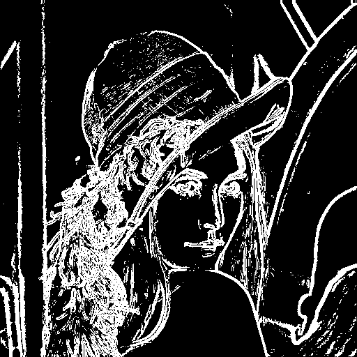
Prewitt 算子梯度图
Prewitt 算子边缘图

1.1.3 Sobel 算子

（1）原理

与 Roberts 算子类似，不过卷积核变为：

$G_x = \begin{bmatrix} -1 & 0 & 1 \\ -2 & 0 & 2 \\ -1 & 0 & 1 \\ \end{bmatrix}$

$G_y = \begin{bmatrix} 1 & 2 & 1 \\ 0 & 0 & 0 \\ -1 & -2 & -1 \\ \end{bmatrix}$

（2）代码

import cv2
import numpy as np
import BASE_DATA

# 定义Sobel算子的卷积核
kernel_x = np.array([[-1, 0, 1],
                     [-2, 0, 2],
                     [-1, 0, 1]])
kernel_y = np.array([[1, 2, 1],
                     [0, 0, 0],
                     [-1, -2, -1]])

def Sobel_operator(image_path=BASE_DATA.IMAGE_PATH, threshold=BASE_DATA.THRESHOLD):
    # 读取灰度图像
    image = cv2.imread(image_path, cv2.IMREAD_GRAYSCALE)
    image_16 = image.astype(np.int16)

    # 计算梯度
    gradient_x = cv2.filter2D(image_16, -1, kernel_x)
    gradient_y = cv2.filter2D(image_16, -1, kernel_y)

    # 计算梯度的近似绝对值
    gradient_magnitude = np.clip(np.abs(gradient_x) + np.abs(gradient_y), 0, 255).astype(np.uint8)

    # 应用阈值处理
    edges = np.zeros_like(gradient_magnitude)
    edges[gradient_magnitude > threshold] = 255

    # 显示结果
    cv2.imshow('Original grayscale image', image)
    cv2.imshow('Gradient image', gradient_magnitude)
    cv2.imshow('Edge image', edges)

    cv2.waitKey(0)
    cv2.destroyAllWindows()

    return edges

if __name__ == '__main__':
    image_path = BASE_DATA.IMAGE_PATH
    edges = Sobel_operator(image_path, BASE_DATA.THRESHOLD)
    # 保存边缘检测结果到文件
    out_path = BASE_DATA.RESULT_DIR + r'\Sobel.png'
    cv2.imwrite(out_path, edges)

（3）结果

Sobel 算子梯度图
Sobel 算子边缘图

（4）优缺点

对像素位置的影响做了加权，比 Prewitt 算子、Roberts 算子效果更好。

（5）Python 函数

Python 提供了 Sobel() 函数进行运算，代码如下：
cv.Sobel( src, ddepth, dx, dy[, dst[, ksize[, scale[, delta[, borderType]]]]] ) -> dst

使用如下，

gradient_x = cv2.Sobel(image, cv2.CV_16S, 1, 0, ksize=3)

gradient_y = cv2.Sobel(image, cv2.CV_16S, 0, 1, ksize=3)

Sobel 算子核

当 dx = 1 且 dy = 0 时，使用以下核来计算 x 方向的一阶导数：
```
[-1, 0, 1]
[-2, 0, 2]
[-1, 0, 1]
```
当 dx = 0 且 dy = 1 时，使用以下核来计算 y 方向的一阶导数：
```
[1, 2, 1]
[0, 0, 0]
[-1, -2, -1]
```

整体代码。

import cv2
import numpy as np
import BASE_DATA

def Sobel_operator(image_path=BASE_DATA.IMAGE_PATH, threshold=BASE_DATA.THRESHOLD):
    # 读取灰度图像
    image = cv2.imread(image_path, cv2.IMREAD_GRAYSCALE)

    # 使用 cv2.Sobel() 计算 x 和 y 方向的梯度
    gradient_x = cv2.Sobel(image, cv2.CV_16S, 1, 0, ksize=3)
    gradient_y = cv2.Sobel(image, cv2.CV_16S, 0, 1, ksize=3)

    # 计算梯度的近似绝对值
    gradient_magnitude = np.clip(np.abs(gradient_x) + np.abs(gradient_y), 0, 255).astype(np.uint8)

    # 应用阈值处理
    edges = np.zeros_like(gradient_magnitude)
    edges[gradient_magnitude > threshold] = 255

    # 显示结果
    cv2.imshow('Original grayscale image', image)
    cv2.imshow('Gradient image', gradient_magnitude)
    cv2.imshow('Edge image', edges)

    cv2.waitKey(0)
    cv2.destroyAllWindows()

    return edges


if __name__ == '__main__':
    image_path = BASE_DATA.IMAGE_PATH
    edges = Sobel_operator(image_path, BASE_DATA.THRESHOLD)
    # 保存边缘检测结果到文件
    out_path = BASE_DATA.RESULT_DIR + r'\Sobel.png'
    cv2.imwrite(out_path, edges)