


实验目标
本实验旨在通过实现一个基础的决策树分类模型,帮助掌握以下技能:理解并应用决策树分类模型:学习如何使用Scikit-learn库的DecisionTreeClassifier来实现分类任务。数据集划分与训练:掌握如何将数据划分为训练集和测试集,并进行模型训练。模型调优:通过测试不同深度的决策树,理解树的深度对模型性能的影响,并找到最佳深度。模型评估与可视化:评估决策树模型的准确率,学习如何通过可视化工具展示决策树及其规则。
实验环境
o Python 3.x
o Scikit-learn、NumPy和Pandas库
o Jupyter Notebook
o Matplotlib
实验数据集
本实验使用的是鸢尾花数据集(Iris dataset),它是一个经典的多分类数据集,包含150个样本,4个特征(花萼长度、花萼宽度、花瓣长度、花瓣宽度),以及3个目标类别(Setosa、Versicolor、Virginica)。
实验步骤
一、导入必要的库
import numpy as np
import matplotlib.pyplot as plt
from sklearn.datasets import load_iris
from sklearn.model_selection import train_test_split
from sklearn.tree import DecisionTreeClassifier, export_text, plot_tree
from sklearn.metrics import accuracy_score
import matplotlib  # 设置中文字体
matplotlib.rcParams['font.sans-serif'] = ['SimHei']    # SimHei 是常用的中文黑体字体
matplotlib.rcParams['axes.unicode_minus'] = False    # 显示负号
二、加载数据集,并划分训练集和测试集
data = load_iris()
X = data.data
y = data.target


print("特征数据形状:", X.shape)
print("目标标签的分布:", np.bincount(y))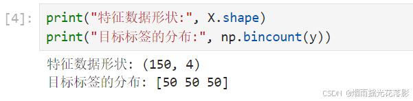
三、数据划分:分为训练集和测试集,测试集占比为 20%
X_train, X_test, y_train, y_test = train_test_split(X, y, test_size=0.2, random_state=42)四、基础模型训练:使用默认深度的决策树分类器
clf = DecisionTreeClassifier(random_state=42)
clf.fit(X_train, y_train)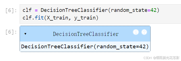
五、预测和评估模型的基础准确率
y_pred = clf.predict(X_test)  # 在测试集上进行预测
accuracy = accuracy_score(y_test, y_pred)
print(f"基础决策树准确率: {accuracy:.2f}")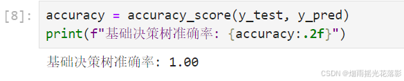
六、可视化基础决策树
plt.figure(figsize=(12, 8))
plot_tree(clf, filled=True, feature_names=data.feature_names, class_names=data.target_names, rounded=True)
plt.title("基础决策树可视化")
plt.show()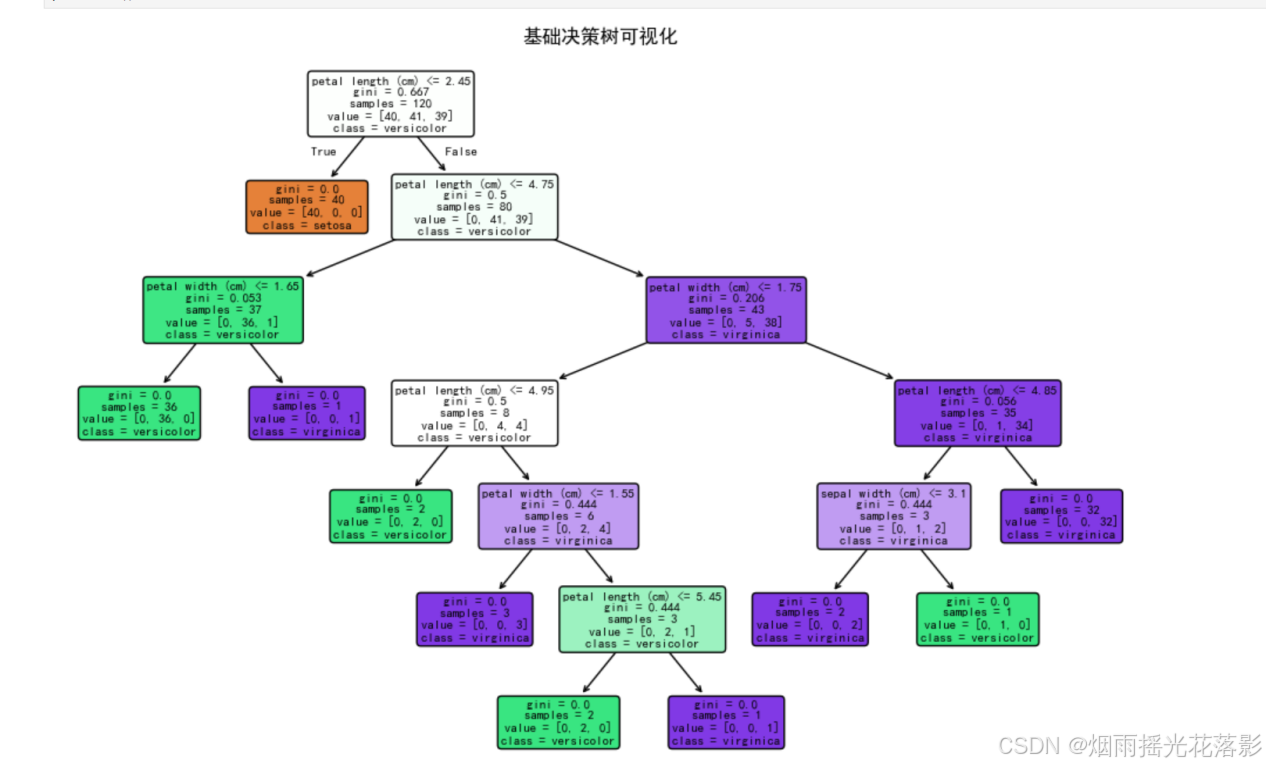
七、打印决策树的规则
tree_rules = export_text(clf, feature_names=data.feature_names)
print("基础决策树规则:\n", tree_rules)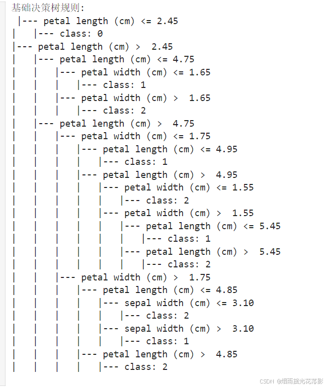
八、深度优化实验:测试不同深度下的准确率
train_accuracies = []
test_accuracies = []
depth_range = range(1, 11)
九、遍历不同的深度值且计算训练集和测试集的准确率
for depth in depth_range:
    clf = DecisionTreeClassifier(max_depth=depth, random_state=42)
    clf.fit(X_train, y_train)
    # 计算训练集和测试集的准确率
    train_accuracy = clf.score(X_train, y_train)
    test_accuracy = clf.score(X_test, y_test)
    train_accuracies.append(train_accuracy)
test_accuracies.append(test_accuracy)
十、绘制深度与准确率的关系图
plt.figure(figsize=(10, 6))
plt.plot(depth_range, train_accuracies, label="训练集准确率", marker='o')
plt.plot(depth_range, test_accuracies, label="测试集准确率", marker='o')
plt.xlabel("树的深度")
plt.ylabel("准确率")
plt.title("不同深度下的训练与测试准确率")
plt.legend()
plt.grid(True)
plt.show()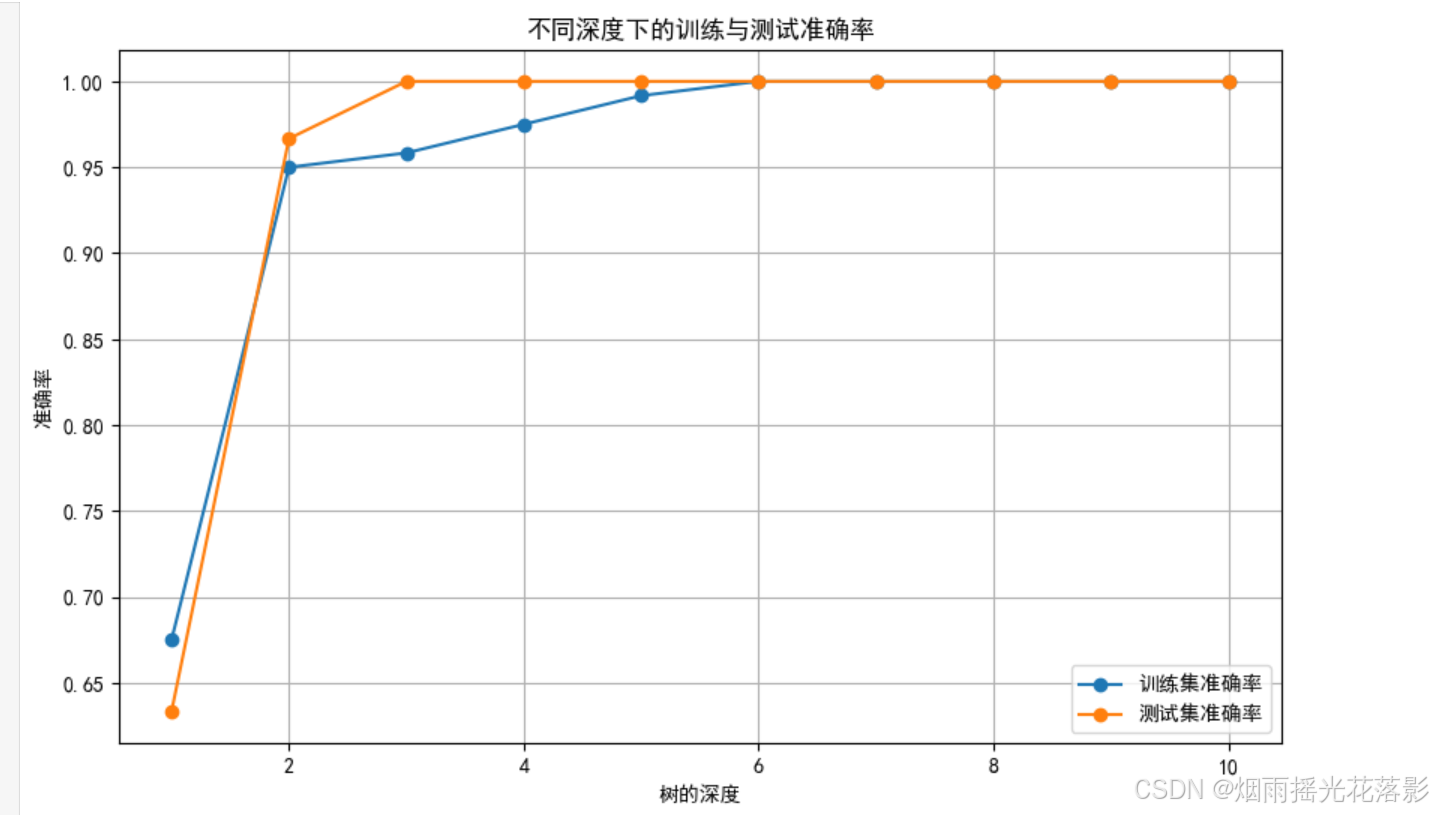
十一、找到测试集准确率最高的深度
best_depth = depth_range[np.argmax(test_accuracies)]
print(f"最佳决策树深度: {best_depth}")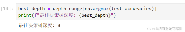
十二、使用最佳深度重新训练决策树
clf_best = DecisionTreeClassifier(max_depth=best_depth, random_state=42)
clf_best.fit(X_train, y_train)
十三、计算并打印最佳深度模型的准确率
y_pred_best = clf_best.predict(X_test)
accuracy_best = accuracy_score(y_test, y_pred_best)
print(f"最佳深度模型在测试集上的准确率: {accuracy_best:.2f}")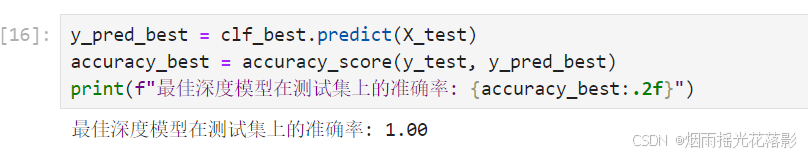
十四、可视化最佳深度的决策树
plt.figure(figsize=(12, 8))
plot_tree(clf_best,filled=True,feature_names=data.feature_names,class_names=data.target_names, rounded=True)
plt.title(f"最佳深度决策树可视化(深度={best_depth})")
plt.show()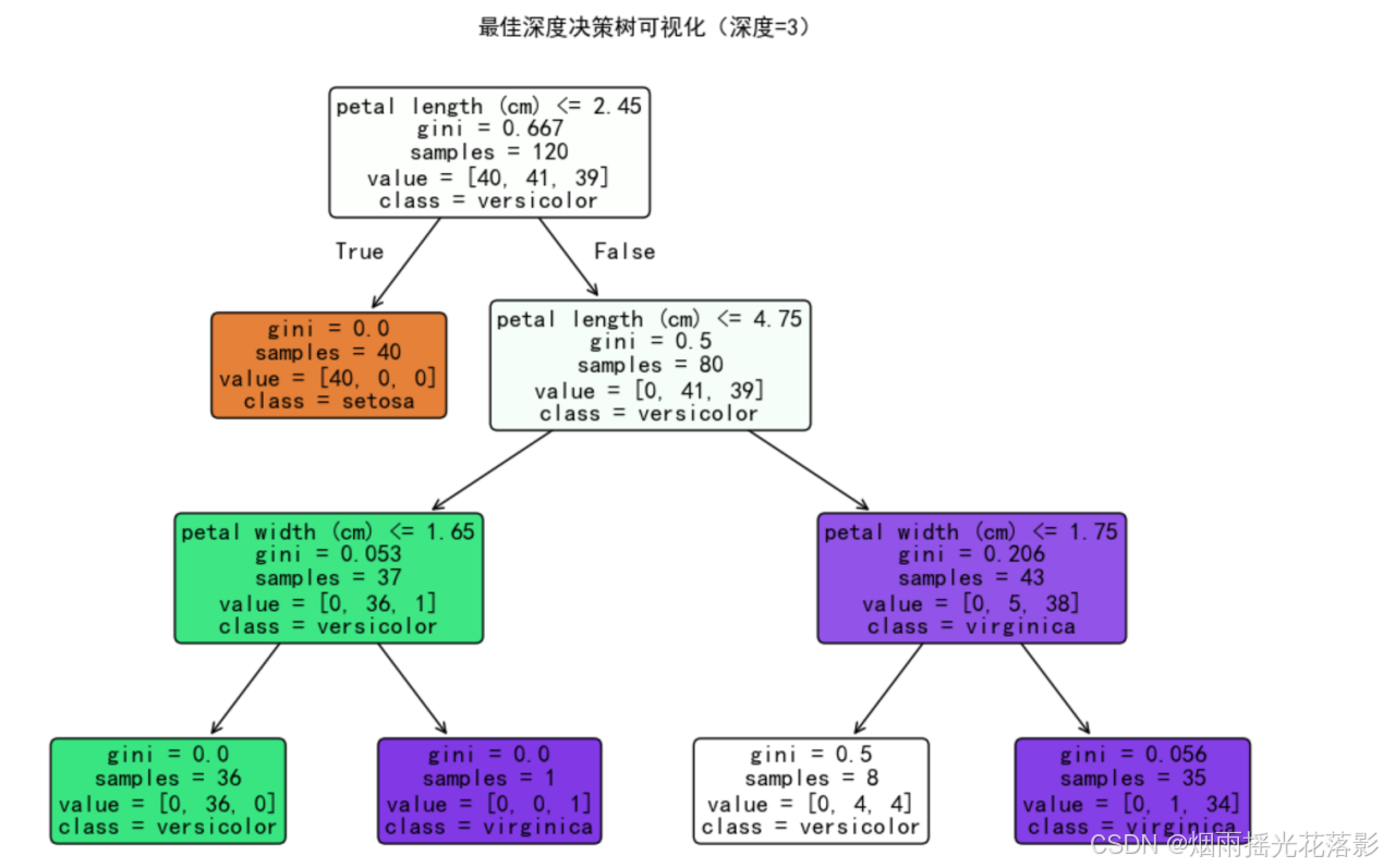
十五、打印最佳深度的决策树规则
tree_rules_best = export_text(clf_best, feature_names=data.feature_names)
print(f"最佳深度决策树规则:\n", tree_rules_best)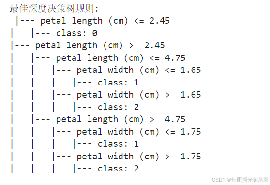


 被折叠的 条评论
为什么被折叠?
被折叠的 条评论
为什么被折叠?
 到【灌水乐园】发言


