


基本变换
1 基向量的变换
1.1 基向量的变换
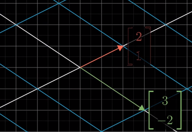
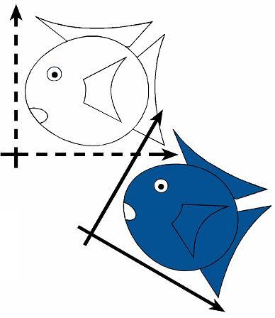
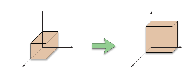
初始基向量为 i ^ ( 1 , 0 ) , j ^ ( 0 , 1 ) \hat{i}(1,0),\hat{j}(0,1) i^(1,0),j^(0,1),经过变换后变为 i ^ ( 3 , − 2 ) , j ^ ( 2 , 1 ) \hat{i}(3,-2), \hat{j}(2,1) i^(3,−2),j^(2,1)

1.2 线性变换对向量的作用
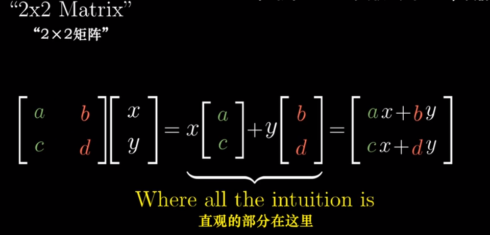
仅需取出向量的坐标,将它们分别于矩阵的特定列相乘,然后将结果相加即可
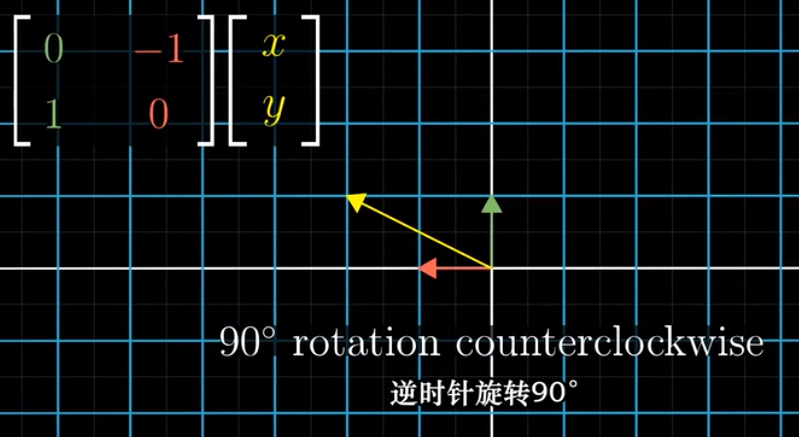
逆时针旋转90°的例子
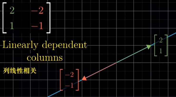
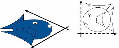
当两个向量变为线性相关时,两个向量共线,二维空间会被挤压到一维
2 Transformation Classification(分类)
2.1 Rigid-body Transformation (刚体变换)
物体本身的长度、角度、大小不会变化包括:
- Identity(不变)
- Translation(平移)
- Rotation(旋转)
- 以及他们的组合
2.2 Similarity Transformation(相似变换)
保持角度
- Identity(不变)
- Translation(平移)
- Rotation(旋转)
- Isotropic Scaling(均衡缩放)
- 以及他们的组合
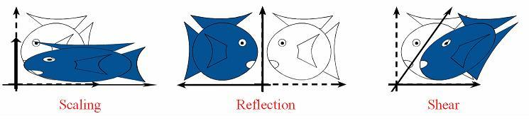
2.3 Linear Transformation(线性变换)
线性变换满足如下方程:
L(p + q) = L(p) + L(q)

aL(p) = L(ap)
- Identity(不变)
- Rotation(旋转)
- Scaling(缩放)
- Reflection(对称)
- Shear(切变、剪切)
2.4 Affine Transformation(仿射变换)
保持直线以及直线与直线的平行
- 线性变换
- 相似变换
- 以及它们的组合
2.5 Projective Transformation(投影变换)
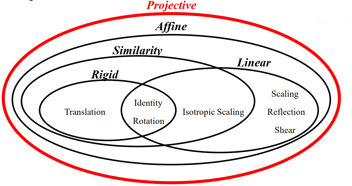
- Grid lines remain parallel and evenly spaced and such that the origin remains fixed.
- 它保持网格线平行且等距分布,并且保持原点不动
3 Homogeneous Coordinates(齐次坐标)
- The objective of HC is to use a 4D column matrices to represent both points and vectors in 3D
- 齐次坐标的本质是使用四维数组来表示三维空间中的点和向量
- If we multiply a homogeneous coordinate by an affine matrix, w is unchanged; by an projective matrix, the value of w will change
- w=0时齐次坐标表示一个方向而不是一个点
3.1 Translate
[ x ′ y ′ z ′ 1 ] = [ 1 0 0 t x 0 1 0 t y 0 0 1 t z 0 0 0 1 ] ⋅ [ x y z 1 ] \begin{bmatrix} x'\\ y'\\ z' \\ 1 \end{bmatrix} = \begin{bmatrix} 1 & 0 & 0 & t_x\\ 0 & 1 & 0 & t_y\\ 0 & 0 & 1 & t_z\\ 0 & 0 & 0 & 1 \end{bmatrix}\cdot \begin{bmatrix} x\\ y\\ z\\ 1 \end{bmatrix} ⎣⎢⎢⎡x′y′z′1⎦⎥⎥⎤=⎣⎢⎢⎡100001000010txtytz1⎦⎥⎥⎤⋅⎣⎢⎢⎡xyz1⎦⎥⎥⎤
3.2 Scale
P ′ = [ a 0 0 0 b 0 0 0 a ] ⋅ [ P x P y P z ] P' = \begin{bmatrix} a & 0 & 0\\ 0 & b & 0\\ 0 & 0 & a \end{bmatrix}\cdot \begin{bmatrix} P_x\\ P_y\\ P_z \end{bmatrix} P′=⎣⎡a000b000a⎦⎤⋅⎣⎡PxPyPz⎦⎤
3.3 Rotation
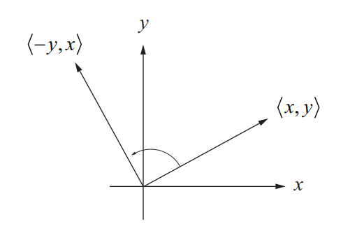
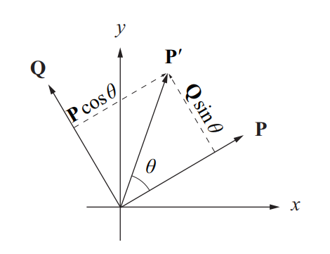
取[-y, x]为Q作为垂直于P的向量,则:
P
′
=
P
c
o
s
θ
+
Q
s
i
n
θ
P' = Pcos\theta + Q sin\theta
P′=Pcosθ+Qsinθ
{
P
x
′
=
P
x
c
o
s
θ
−
P
y
s
i
n
θ
P
y
′
=
P
y
c
o
s
θ
+
P
x
s
i
n
θ
\left\{\begin{matrix} P_x' = P_xcos\theta - P_ysin\theta\\ P_y' = P_ycos\theta + P_xsin\theta \end{matrix}\right.
{Px′=Pxcosθ−PysinθPy′=Pycosθ+Pxsinθ
P
′
=
[
c
o
s
θ
−
s
i
n
θ
s
i
n
θ
c
o
s
θ
]
P
P' = \begin{bmatrix} cos\theta & -sin\theta\\ sin\theta & cos\theta\\ \end{bmatrix}P
P′=[cosθsinθ−sinθcosθ]P
R
z
(
θ
)
=
[
c
o
s
θ
−
s
i
n
θ
0
s
i
n
θ
c
o
s
θ
0
0
0
1
]
R_z(\theta) = \begin{bmatrix} cos\theta & -sin\theta & 0\\ sin\theta & cos\theta & 0\\ 0 & 0 & 1\\ \end{bmatrix}
Rz(θ)=⎣⎡cosθsinθ0−sinθcosθ0001⎦⎤
R
x
(
θ
)
=
[
1
0
0
0
c
o
s
θ
−
s
i
n
θ
0
s
i
n
θ
c
o
s
θ
]
R_x(\theta) = \begin{bmatrix} 1 & 0 & 0\\ 0 & cos\theta & -sin\theta\\ 0 & sin\theta & cos\theta\\ \end{bmatrix}
Rx(θ)=⎣⎡1000cosθsinθ0−sinθcosθ⎦⎤
R
y
(
θ
)
=
[
c
o
s
θ
0
s
i
n
θ
0
1
0
−
s
i
n
θ
0
c
o
s
θ
]
R_y(\theta) = \begin{bmatrix} cos\theta & 0 & sin\theta\\ 0 & 1 & 0\\ -sin\theta & 0 & cos\theta\\ \end{bmatrix}
Ry(θ)=⎣⎡cosθ0−sinθ010sinθ0cosθ⎦⎤
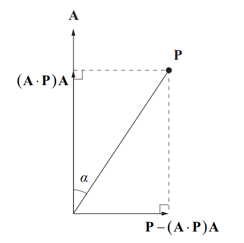
3.4 Rotation About an Arbitrary Axis
p r o j A P = ( A ⋅ P ) A p e r p A P = P − ( A ⋅ P ) A proj_AP = (A\cdot P)A\\ perp_AP = P - (A\cdot P)A projAP=(A⋅P)AperpAP=P−(A⋅P)A
因为与A重合的旋转后不会改变,所以仅需计算垂直的向量即可。为了计算 p e r p A P perp_AP perpAP的旋转,需要先得到与其垂直的向量,即 A × P A\times P A×P
rotation of
p
e
r
p
A
P
perp_AP
perpAP through an angle θ as
P
′
=
[
P
−
(
A
⋅
P
)
A
]
c
o
s
θ
+
(
A
×
P
)
s
i
n
θ
+
(
A
⋅
P
)
A
P' = [P - (A\cdot P)A]cos\theta + (A \times P)sin\theta + (A\cdot P)A
P′=[P−(A⋅P)A]cosθ+(A×P)sinθ+(A⋅P)A
3.5 Transforming Normal Vectors
We could find that translation, rotation and isotropic scale preserve the correct normal, but shear or isotropic scale will make the normal incorrect.
If M is a 3×3 matrix with which we transform a vertex position, then the same matrix M
can be used to correctly transform the tangent vector at that vertex.
N , T N,T N,T为变换前的法向量和切向量, N ′ , T ′ N',T' N′,T′为变换后的法向量和切向量,则:
N
⋅
T
=
N
T
T
=
0
N\cdot T = N^T T = 0
N⋅T=NTT=0
N
′
⋅
T
′
=
N
′
T
T
′
=
0
N'\cdot T' = N'^T T' = 0
N′⋅T′=N′TT′=0
N
T
(
M
−
1
M
)
T
=
N
T
M
−
1
T
′
=
0
N^T (M^{-1} M)T = N^TM^{-1} T'= 0
NT(M−1M)T=NTM−1T′=0
N
′
T
=
N
T
M
−
1
N'^T = N^TM^{-1}
N′T=NTM−1
N
′
=
(
M
−
1
)
T
N
N' = (M^{-1})^T N
N′=(M−1)TN
So the matrix is the transpose of inverse of M
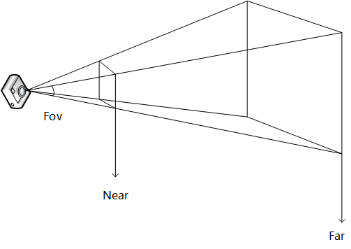
4 Projection
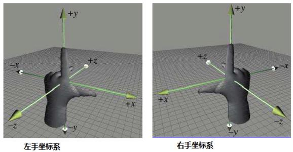
大拇指指向为x轴正方向,食指指向为y轴正方向,中指指向为z轴正方向,OpenGL采用右手坐标系,DirectX为左手坐标系
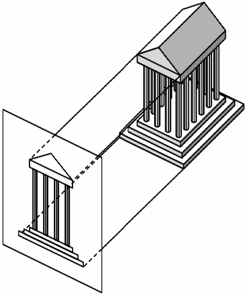
4.1 Orthographic Projection(正交投影)
When the focal point is at infinity, the rays are parallel and orthogonal to the image plane, When xy-plane is the image plane, ( x , y , z ) − > ( x , y , 0 ) \bm{(x,y,z) -> (x,y,0)} (x,y,z)−>(x,y,0)
4.2 正交投影矩阵

为了后续裁剪的方便,我们需要将物体的坐标转换到canonical view volume (CVV) 中,转换后的坐标被称为normalized device coordinates (NDC),这里l,r,b,t,n,f采用对应的x轴y轴z轴坐标值。投影就是将长方形的视域体压缩到指定范围即可,从x轴开始,视域体中的点的x坐标范围在[l, r],想把它变换到范围在[-1, 1]:
l ⩽ x ⩽ r 0 ⩽ x − l ⩽ r − l 0 ⩽ x − l r − l ⩽ 1 − 1 ⩽ 2 ( x − l ) r − l − 1 ⩽ 1 − 1 ⩽ 2 x r − l − r + l r − l ⩽ 1 x ′ = 2 r − l x − r + l r − l l\leqslant x \leqslant r \\ 0\leqslant x - l \leqslant r - l \\ 0\leqslant \frac{x - l}{r - l} \leqslant 1 \\ -1\leqslant \frac{2(x - l)}{r - l} - 1 \leqslant 1 \\ -1\leqslant \frac{2x}{r - l} - \frac{r + l}{r - l} \leqslant 1 \\ x' = \frac{2}{r - l}x - \frac{r + l}{r - l} l⩽x⩽r0⩽x−l⩽r−l0⩽r−lx−l⩽1−1⩽r−l2(x−l)−1⩽1−1⩽r−l2x−r−lr+l⩽1x′=r−l2x−r−lr+l
y同理
y
′
=
2
t
−
b
y
−
t
+
b
t
−
b
y' = \frac{2}{t - b}y - \frac{t + b}{t - b}
y′=t−b2y−t−bt+b
z需要在z=n时映射为-1,z=f时映射为1
−
1
=
n
A
+
B
1
=
f
A
+
B
A
=
2
f
−
n
B
=
−
f
+
n
f
−
n
-1 = nA + B \\ 1 = fA + B \\ A = \frac{2}{f - n} \\ B = -\frac{f + n}{f - n} \\
−1=nA+B1=fA+BA=f−n2B=−f−nf+n
所以z’为
z ′ = 2 f − n z − f + n f − n z' = \frac{2}{f - n}z - \frac{f + n}{f - n} z′=f−n2z−f−nf+n
所以正交投影矩阵为
[ 2 r − l 0 0 − r + l r − l 0 2 t − b 0 − t + b t − b 0 0 2 f − n − f + n f − n 0 0 0 1 ] \begin{bmatrix} \frac{2}{r - l} & 0 & 0 & -\frac{r + l}{r - l}\\ 0 & \frac{2}{t - b} & 0 & -\frac{t + b}{t - b}\\ 0 & 0 & \frac{2}{f - n} & -\frac{f + n}{f - n}\\ 0 & 0 & 0 & 1 \end{bmatrix} ⎣⎢⎢⎡r−l20000t−b20000f−n20−r−lr+l−t−bt+b−f−nf+n1⎦⎥⎥⎤
通常情况下摄像机定位在原点并且沿着z轴方向观看,所以l与r,b与t是轴对称的,我们可以定义宽度为w = r - l,高度为h = t - b,矩阵可以简化为
[ 2 w 0 0 0 0 2 h 0 0 0 0 2 f − n − f + n f − n 0 0 0 1 ] \begin{bmatrix} \frac{2}{w} & 0 & 0 & 0\\ 0 & \frac{2}{h} & 0 & 0\\ 0 & 0 & \frac{2}{f - n} & -\frac{f + n}{f - n}\\ 0 & 0 & 0 & 1 \end{bmatrix} ⎣⎢⎢⎡w20000h20000f−n2000−f−nf+n1⎦⎥⎥⎤
4.2.1 OpenGL正交投影矩阵
在OpenGL中n,f为正值,表示距离相机的远近,所以要对投影矩阵中的n,f取负
[ 2 r − l 0 0 − r + l r − l 0 2 t − b 0 − t + b t − b 0 0 − 2 f − n − f + n f − n 0 0 0 1 ] \begin{bmatrix} \frac{2}{r - l} & 0 & 0 & -\frac{r + l}{r - l}\\ 0 & \frac{2}{t - b} & 0 & -\frac{t + b}{t - b}\\ 0 & 0 & -\frac{2}{f - n} & -\frac{f + n}{f - n}\\ 0 & 0 & 0 & 1 \end{bmatrix} ⎣⎢⎢⎡r−l20000t−b20000−f−n20−r−lr+l−t−bt+b−f−nf+n1⎦⎥⎥⎤
4.2.2 DirectX正交投影矩阵
DirectX坐标轴z轴朝里,且将z值映射为[0,1]所以,DirectX的正交投影矩阵为
[ 2 r − l 0 0 − r + l r − l 0 2 t − b 0 − t + b t − b 0 0 1 f − n − n f − n 0 0 0 1 ] \begin{bmatrix} \frac{2}{r - l} & 0 & 0 & -\frac{r + l}{r - l}\\ 0 & \frac{2}{t - b} & 0 & -\frac{t + b}{t - b}\\ 0 & 0 & \frac{1}{f - n} & -\frac{n}{f - n}\\ 0 & 0 & 0 & 1 \end{bmatrix} ⎣⎢⎢⎡r−l20000t−b20000f−n10−r−lr+l−t−bt+b−f−nn1⎦⎥⎥⎤
4.3 Perspective Projection(透视投影)
When
- The camera is at the origin point and looks along the z-axis
- The image plane is paraellel to the xy-plane at distance d
- ( x , y , z ) − > ( ( − d / z ) x , ( − d / z ) y , d ) \bm{(x,y,z) -> ((-d/z)x, (-d/z)y, d)} (x,y,z)−>((−d/z)x,(−d/z)y,d)
4.4 透视投影矩阵

4.4.1 透视投影矩阵
在透视投影中将点投影的近平面,则x与y的变化如下
x ′ = n z x y ′ = n z y x' = \frac{n}{z}x \\ y' = \frac{n}{z}y \\ x′=znxy′=zny
然后用正交投影的公式,就可以把x和y的坐标转换到[-1, 1]的范围内
x ′ = 2 r − l n z x − r + l r − l y ′ = 2 t − b n z y − t + b t − b x' = \frac{2}{r - l}\frac{n}{z}x - \frac{r + l}{r - l} \\ y' = \frac{2}{t - b}\frac{n}{z}y - \frac{t + b}{t - b}\\ x′=r−l2znx−r−lr+ly′=t−b2zny−t−bt+b
这里有个z,无法直接用矩阵表示,我们可以两边都乘以z
x ′ z = 2 n r − l x − r + l r − l z y ′ z = 2 n t − b y − t + b t − b z x'z = \frac{2n}{r - l}x - \frac{r + l}{r - l}z \\ y'z = \frac{2n}{t - b}y - \frac{t + b}{t - b}z\\ x′z=r−l2nx−r−lr+lzy′z=t−b2ny−t−bt+bz
对于变换后的z’来说,z’并不依赖于x和y,为了统一我们也将z’乘以z,因此z’z = az + b,z=-n时,z’=-1;z=-f时,z’=1,于是z’z如下
z ′ z = f + n f − n z − 2 f n f − n z'z = \frac{f + n}{f - n}z - \frac{2fn}{f - n} z′z=f−nf+nz−f−n2fn
最终透视投影矩阵如下
[ 2 n r − l 0 − r + l r − l 0 0 2 n t − b − t + b t − b 0 0 0 f + n f − n − 2 f n f − n 0 0 1 0 ] \begin{bmatrix} \frac{2n}{r - l} & 0 & -\frac{r + l}{r - l} & 0\\ 0 & \frac{2n}{t - b} & -\frac{t + b}{t - b} & 0\\ 0 & 0 & \frac{f + n}{f - n} & - \frac{2fn}{f - n}\\ 0 & 0 & 1 & 0 \end{bmatrix} ⎣⎢⎢⎡r−l2n0000t−b2n00−r−lr+l−t−bt+bf−nf+n100−f−n2fn0⎦⎥⎥⎤
通过矩阵计算得到的结果是(x’z, y’z, z’z, z)。可以看出,w分量此时等于变换之前的z,然后,你应用通常的步骤去除以齐次坐标,得到(x’, y’, z’, 1)
4.4.2 OpenGL透视投影矩阵
在OpenGL中n,f为正值,表示距离相机的远近,所以要对投影矩阵中的n,f取负
x
′
=
−
n
z
x
y
′
=
−
n
z
y
x' = \frac{-n}{z}x \\ y' = \frac{-n}{z}y\\
x′=z−nxy′=z−ny
这里有个-z,无法直接用矩阵表示,我们可以两边都乘以-z
− x ′ z = 2 n r − l x + r + l r − l z − y ′ z = 2 n t − b y + t + b t − b z − z ′ z = − f + n f − n z − 2 f n f − n -x'z = \frac{2n}{r - l}x + \frac{r + l}{r - l}z \\ -y'z = \frac{2n}{t - b}y + \frac{t + b}{t - b}z \\ -z'z = -\frac{f + n}{f - n}z - \frac{2fn}{f - n} \\ −x′z=r−l2nx+r−lr+lz−y′z=t−b2ny+t−bt+bz−z′z=−f−nf+nz−f−n2fn
最终OpenGL透视投影的矩阵如下
[ 2 n r − l 0 r + l r − l 0 0 2 n t − b t + b t − b 0 0 0 − f + n f − n − 2 f n f − n 0 0 − 1 0 ] \begin{bmatrix} \frac{2n}{r - l} & 0 & \frac{r + l}{r - l} & 0\\ 0 & \frac{2n}{t - b} & \frac{t + b}{t - b} & 0\\ 0 & 0 & -\frac{f + n}{f - n} & - \frac{2fn}{f - n}\\ 0 & 0 & -1 & 0 \end{bmatrix} ⎣⎢⎢⎡r−l2n0000t−b2n00r−lr+lt−bt+b−f−nf+n−100−f−n2fn0⎦⎥⎥⎤
4.4.2 DirectX透视投影矩阵
DirectX坐标轴z轴朝里,且将z值映射为[0,1],因此z’z = az + b,z=n时,z’=0;z=f时,z’=1,于是z’z如下
z ′ z = f f − n z − f n f − n z'z = \frac{f}{f - n}z - \frac{fn}{f - n} z′z=f−nfz−f−nfn
最终DirectX透视投影的矩阵如下
[
2
n
r
−
l
0
−
r
+
l
r
−
l
0
0
2
n
t
−
b
−
t
+
b
t
−
b
0
0
0
f
f
−
n
−
f
n
f
−
n
0
0
1
0
]
\begin{bmatrix} \frac{2n}{r - l} & 0 & -\frac{r + l}{r - l} & 0\\ 0 & \frac{2n}{t - b} & -\frac{t + b}{t - b} & 0\\ 0 & 0 & \frac{f}{f - n} & - \frac{fn}{f - n}\\ 0 & 0 & 1 & 0 \end{bmatrix}
⎣⎢⎢⎡r−l2n0000t−b2n00−r−lr+l−t−bt+bf−nf100−f−nfn0⎦⎥⎥⎤
4.4.3 以FOV表示的透视投影矩阵
2 n t − b = n h 2 = c o t f o v 2 2 n r − l = 2 n w = n h 2 1 a s p e c t = c o t f o v 2 1 a s p e c t a s p e c t = w h \frac{2n}{t - b} = \frac{n}{\frac{h}{2}} = cot\frac{fov}{2}\\ \frac{2n}{r - l} = \frac{2n}{w} = \frac{n}{\frac{h}{2}} \frac{1}{aspect} = cot\frac{fov}{2}\frac{1}{aspect}\\ aspect = \frac{w}{h}\\ t−b2n=2hn=cot2fovr−l2n=w2n=2hnaspect1=cot2fovaspect1aspect=hw
所以矩阵可以表示为
[ c o t f o v 2 a s p e c t 0 0 0 0 c o t f o v 2 0 0 0 0 f + n f − n − 2 f n f − n 0 0 1 0 ] \begin{bmatrix} \frac{cot\frac{fov}{2}}{aspect} & 0 & 0 & 0\\ 0 & cot\frac{fov}{2} & 0 & 0\\ 0 & 0 & \frac{f + n}{f - n} & - \frac{2fn}{f - n}\\ 0 & 0 & 1 & 0 \end{bmatrix} ⎣⎢⎢⎢⎡aspectcot2fov0000cot2fov0000f−nf+n100−f−n2fn0⎦⎥⎥⎥⎤
5 屏幕映射
屏幕映射主要是将裁剪空间内的坐标映射成屏幕坐标,以显示到屏幕上。
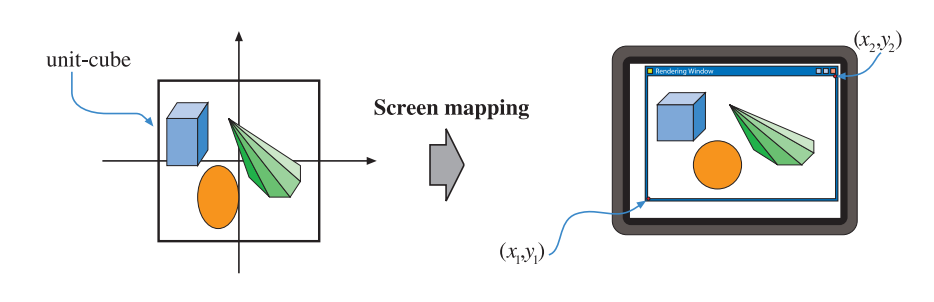
x将从 [ − 1 , 1 ] [-1, 1] [−1,1]映射到 [ x 1 , x 2 ] [x_1, x_2] [x1,x2]
{ − A + B = x 1 A + B = x 2 x ′ = x 2 − x 1 2 x + x 1 + x 2 2 \left\{\begin{matrix} -A + B = x_1\\ A + B = x_2 \end{matrix}\right. \\ x' = \frac{x_2 - x_1}{2}x + \frac{x_1 + x_2}{2} {−A+B=x1A+B=x2x′=2x2−x1x+2x1+x2
同理y’
y
′
=
y
2
−
y
1
2
y
+
y
1
+
y
2
2
y' = \frac{y_2 - y_1}{2}y + \frac{y_1 + y_2}{2}
y′=2y2−y1y+2y1+y2
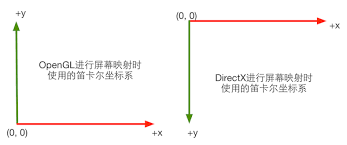
5.1 OpenGL屏幕映射
在OpenGL中 x 1 = 0 , x 2 = w , y 1 = 0 , y 2 = h x_1 = 0, x_2 = w, y_1 = 0, y_2 = h x1=0,x2=w,y1=0,y2=h,所以映射矩阵为
[ w 2 0 0 w 2 0 h 2 0 h 2 0 0 1 0 0 0 0 1 ] \begin{bmatrix} \frac{w}{2} & 0 & 0 & \frac{w}{2}\\ 0 & \frac{h}{2} & 0 & \frac{h}{2}\\ 0 & 0 & 1 & 0\\ 0 & 0 & 0 & 1 \end{bmatrix} ⎣⎢⎢⎡2w00002h0000102w2h01⎦⎥⎥⎤
5.2 DirectX屏幕映射
在DirectX中 x 1 = 0 , x 2 = w , y 1 = h , y 2 = 0 x_1 = 0, x_2 = w, y_1 = h, y_2 = 0 x1=0,x2=w,y1=h,y2=0,所以映射矩阵为
[ w 2 0 0 w 2 0 − h 2 0 h 2 0 0 1 0 0 0 0 1 ] \begin{bmatrix} \frac{w}{2} & 0 & 0 & \frac{w}{2}\\ 0 & -\frac{h}{2} & 0 & \frac{h}{2}\\ 0 & 0 & 1 & 0\\ 0 & 0 & 0 & 1 \end{bmatrix} ⎣⎢⎢⎡2w0000−2h0000102w2h01⎦⎥⎥⎤


 被折叠的 条评论
为什么被折叠?
被折叠的 条评论
为什么被折叠?
 到【灌水乐园】发言


