《动手学深度学习》笔记

task02:文本预处理、语言模型和循环神经网络基础

1.文本预处理

对于文本数据来说，预处理通常包括四个步骤：

1. 读入文本
2. 分词
3. 建立字典，将每个词映射到一个唯一的索引。
4. 将文本从词的序列转换为索引的序列，方便输入模型。

以英文小说Time Machine为例，展示文本预处理的过程

在import collections
import re

def read_time_machine():
    with open('/home/kesci/input/timemachine7163/timemachine.txt', 'r') as f:
        lines = [re.sub('[^a-z]+', ' ', line.strip().lower()) for line in f]
    return lines


lines = read_time_machine()
print('# sentences %d' % len(lines))这里插入代码片

分词
上述操作我们得到了若干个句子，要对句子进行分词操作，也就是将每个句子划分成若干个词(token）,转换为一个词的序列。

def tokenize(sentences, token='word'):
    """Split sentences into word or char tokens"""
    if token == 'word':
        return [sentence.split(' ') for sentence in sentences]
    elif token == 'char':
        return [list(sentence) for sentence in sentences]
    else:
        print('ERROR: unkown token type '+token)

tokens = tokenize(lines)
tokens[0:2]

建立字典
为了使模型处理起来更方便，需要将字符串转换为数字。所以首先构建一个字典（vocabulary）,将每个词映射到唯一的索引编号。

class Vocab(object):
    def __init__(self, tokens, min_freq=0, use_special_tokens=False):
        counter = count_corpus(tokens)  # : 
        self.token_freqs = list(counter.items())
        self.idx_to_token = []
        if use_special_tokens:
            # padding, begin of sentence, end of sentence, unknown
            self.pad, self.bos, self.eos, self.unk = (0, 1, 2, 3)
            self.idx_to_token += ['', '', '', '']
        else:
            self.unk = 0
            self.idx_to_token += ['']
        self.idx_to_token += [token for token, freq in self.token_freqs
                        if freq >= min_freq and token not in self.idx_to_token]
        self.token_to_idx = dict()
        for idx, token in enumerate(self.idx_to_token):
            self.token_to_idx[token] = idx

    def __len__(self):
        return len(self.idx_to_token)

    def __getitem__(self, tokens):
        if not isinstance(tokens, (list, tuple)):
            return self.token_to_idx.get(tokens, self.unk)
        return [self.__getitem__(token) for token in tokens]

    def to_tokens(self, indices):
        if not isinstance(indices, (list, tuple)):
            return self.idx_to_token[indices]
        return [self.idx_to_token[index] for index in indices]

def count_corpus(sentences):
    tokens = [tk for st in sentences for tk in st]
    return collections.Counter(tokens)  # 返回一个字典，记录每个词的出现次数
    ```
```python
vocab = Vocab(tokens)
print(list(vocab.token_to_idx.items())[0:10])

将词转为索引
利用字典，可以将原文本中的句子从单词索引转换为索引序列。

for i in range(8, 10):
    print('words:', tokens[i])
    print('indices:', vocab[tokens[i]])
  

用现有工具进行分词
刚才介绍的分词方式较为简单，一些标点符号通常可以提供语义信息，但是刚才的方法都将其直接丢弃了；许多称呼词也会被错误的处理。现有的一些分词工具可以很好的进行分词，比如NLTK和spaCy

举个例子：Mr. Chen doesn’t agree with my suggestion.

text = "Mr. Chen doesn't agree with my suggestion."

用spaCy

import spacy
nlp = spacy.load('en_core_web_sm')
doc = nlp(text)
print([token.text for token in doc])
['Mr.', 'Chen', 'does', "n't", 'agree', 'with', 'my', 'suggestion', '.']

用NLTK

from nltk.tokenize import word_tokenize
from nltk import data
data.path.append('/home/kesci/input/nltk_data3784/nltk_data')
print(word_tokenize(text))

2.语言模型

主要介绍n元语法
利用马尔可夫假设来简化模型，即指一个词的出现只与前面n个词相关，即n阶马尔可夫链。
假如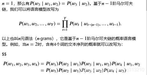

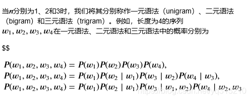
n元语法中，n较小时，语法并不准确；n较大时，需要统计大量词频，导致参数空间过大，出现数稀疏的问题。

下面介绍对时序数据采样的两种方式：随机采样和相邻采样
随机采样
每次从数据中随机采样一个小批量。其中批量大小batch_size是每个小批量的样本数，num_step是每个样本所包含的时间步数。在随机采样中，每个样本是原始序列上任意截取的一段序列，相邻的两个随机小批量在原始序列上的位置不一定相邻。

import torch
import random
def data_iter_random(corpus_indices, batch_size, num_steps, device=None):
    # 减1是因为对于长度为n的序列，X最多只有包含其中的前n - 1个字符
    num_examples = (len(corpus_indices) - 1) // num_steps  # 下取整，得到不重叠情况下的样本个数
    example_indices = [i * num_steps for i in range(num_examples)]  # 每个样本的第一个字符在corpus_indices中的下标
    random.shuffle(example_indices)

    def _data(i):
        # 返回从i开始的长为num_steps的序列
        return corpus_indices[i: i + num_steps]
    if device is None:
        device = torch.device('cuda' if torch.cuda.is_available() else 'cpu')
    
    for i in range(0, num_examples, batch_size):
        # 每次选出batch_size个随机样本
        batch_indices = example_indices[i: i + batch_size]  # 当前batch的各个样本的首字符的下标
        X = [_data(j) for j in batch_indices]
        Y = [_data(j + 1) for j in batch_indices]
        yield torch.tensor(X, device=device), torch.tensor(Y, device=device)

输入0-29的连续整数作为一个序列，设批量大小和时间步数分别为2和6，打印随机采样每次读取的小批量样本的输入X和标签Y。

my_seq = list(range(30))
for X, Y in data_iter_random(my_seq, batch_size=2, num_steps=6):
    print('X: ', X, '\nY:', Y, '\n')

输出结果为：

X:  tensor([[ 6,  7,  8,  9, 10, 11],
        [12, 13, 14, 15, 16, 17]]) 
Y: tensor([[ 7,  8,  9, 10, 11, 12],
        [13, 14, 15, 16, 17, 18]]) 

X:  tensor([[ 0,  1,  2,  3,  4,  5],
        [18, 19, 20, 21, 22, 23]]) 
Y: tensor([[ 1,  2,  3,  4,  5,  6],
        [19, 20, 21, 22, 23, 24]])

相邻采样
即相邻的两个随机小批量在原始序列上的位置相毗邻，给我的感觉跟希尔排序有点类似。

def data_iter_consecutive(corpus_indices, batch_size, num_steps, device=None):
    if device is None:
        device = torch.device('cuda' if torch.cuda.is_available() else 'cpu')
    corpus_len = len(corpus_indices) // batch_size * batch_size  # 保留下来的序列的长度
    corpus_indices = corpus_indices[: corpus_len]  # 仅保留前corpus_len个字符
    indices = torch.tensor(corpus_indices, device=device)
    indices = indices.view(batch_size, -1)  # resize成(batch_size, )
    batch_num = (indices.shape[1] - 1) // num_steps
    for i in range(batch_num):
        i = i * num_steps
        X = indices[:, i: i + num_steps]
        Y = indices[:, i + 1: i + num_steps + 1]
        yield X, Y

依旧用0-29作为输入，批量大小和时间步数分别为2和6

for X, Y in data_iter_consecutive(my_seq, batch_size=2, num_steps=6):
    print('X: ', X, '\nY:', Y, '\n')

输出结果为：

X:  tensor([[ 0,  1,  2,  3,  4,  5],
        [15, 16, 17, 18, 19, 20]]) 
Y: tensor([[ 1,  2,  3,  4,  5,  6],
        [16, 17, 18, 19, 20, 21]]) 

X:  tensor([[ 6,  7,  8,  9, 10, 11],
        [21, 22, 23, 24, 25, 26]]) 
Y: tensor([[ 7,  8,  9, 10, 11, 12],
        [22, 23, 24, 25, 26, 27]]) 

3.循环神经网络基础（RNN）

1. 裁剪梯度：RNN中较容易出现梯度衰减或者梯度爆炸，导致网络无法训练。裁剪梯度是一种应对梯度爆炸的方法。
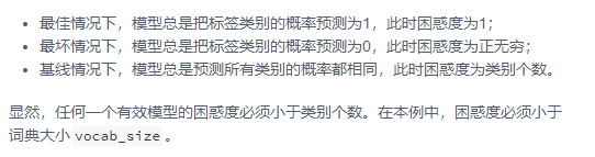
2. 困惑度：是对交叉熵损失函数做指数运算后得到的值。
   
   下面是函数rnn用循环的方式一次完成循环神经网络的每个时间步的计算

def rnn(inputs, state, params):
    # inputs和outputs皆为num_steps个形状为(batch_size, vocab_size)的矩阵
    W_xh, W_hh, b_h, W_hq, b_q = params
    H, = state
    outputs = []
    for X in inputs:
        H = torch.tanh(torch.matmul(X, W_xh) + torch.matmul(H, W_hh) + b_h)
        Y = torch.matmul(H, W_hq) + b_q
        outputs.append(Y)
    return outputs, (H,)

在训练函数中需要注意几点：

1. 使用困惑度评价模型
2. 在迭代模型参数前裁剪梯度
3. 如果采用不同的采样方法，将会导致隐藏状态初始化不同

训练函数

def train_and_predict_rnn(rnn, get_params, init_rnn_state, num_hiddens,
                          vocab_size, device, corpus_indices, idx_to_char,
                          char_to_idx, is_random_iter, num_epochs, num_steps,
                          lr, clipping_theta, batch_size, pred_period,
                          pred_len, prefixes):
    if is_random_iter:
        data_iter_fn = d2l.data_iter_random
    else:
        data_iter_fn = d2l.data_iter_consecutive
    params = get_params()
    loss = nn.CrossEntropyLoss()

    for epoch in range(num_epochs):
        if not is_random_iter:  # 如使用相邻采样，在epoch开始时初始化隐藏状态
            state = init_rnn_state(batch_size, num_hiddens, device)
        l_sum, n, start = 0.0, 0, time.time()
        data_iter = data_iter_fn(corpus_indices, batch_size, num_steps, device)
        for X, Y in data_iter:
            if is_random_iter:  # 如使用随机采样，在每个小批量更新前初始化隐藏状态
                state = init_rnn_state(batch_size, num_hiddens, device)
            else:  # 否则需要使用detach函数从计算图分离隐藏状态
                for s in state:
                    s.detach_()
            # inputs是num_steps个形状为(batch_size, vocab_size)的矩阵
            inputs = to_onehot(X, vocab_size)
            # outputs有num_steps个形状为(batch_size, vocab_size)的矩阵
            (outputs, state) = rnn(inputs, state, params)
            # 拼接之后形状为(num_steps * batch_size, vocab_size)
            outputs = torch.cat(outputs, dim=0)
            # Y的形状是(batch_size, num_steps)，转置后再变成形状为
            # (num_steps * batch_size,)的向量，这样跟输出的行一一对应
            y = torch.flatten(Y.T)
            # 使用交叉熵损失计算平均分类误差
            l = loss(outputs, y.long())
            
            # 梯度清0
            if params[0].grad is not None:
                for param in params:
                    param.grad.data.zero_()
            l.backward()
            grad_clipping(params, clipping_theta, device)  # 裁剪梯度
            d2l.sgd(params, lr, 1)  # 因为误差已经取过均值，梯度不用再做平均
            l_sum += l.item() * y.shape[0]
            n += y.shape[0]

        if (epoch + 1) % pred_period == 0:
            print('epoch %d, perplexity %f, time %.2f sec' % (
                epoch + 1, math.exp(l_sum / n), time.time() - start))
            for prefix in prefixes:
                print(' -', predict_rnn(prefix, pred_len, rnn, params, init_rnn_state,
                    num_hiddens, vocab_size, device, idx_to_char, char_to_idx))

若使用相邻采样，在epoch开始时初始化隐藏状态;若使用随机采样，在每个小批量更新前初始化