


 本文深入探讨支持向量机(SVM)原理,涵盖线性与非线性分类,软边际与正则化概念,以及SVM在sklearn中的实现与应用,包括回归问题的解决。
1、支持向量机
可以解决分类问题,也可以解决回归问题
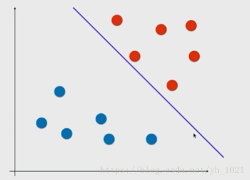
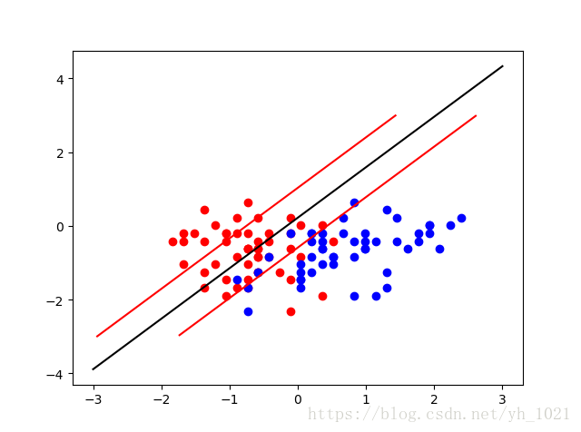
在上图所示中,有两类数据,如果使用逻辑回归,那在两组数据中找出一条分界线即可,当然这个分界线有很多种可能。如果有一个新的数据,是靠近红色点的那一边,但是没有过线而被分为了蓝色点,在这种情况下的模型的泛化能力是不高的。
我们选择另一条分割线,使得两组数据距离直线的最近距离相等,这样的模型泛化能力较高。
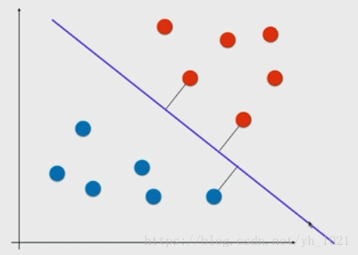
再画出两条与分割线相平行的直线,使得在这两条直线当中没有数据点。
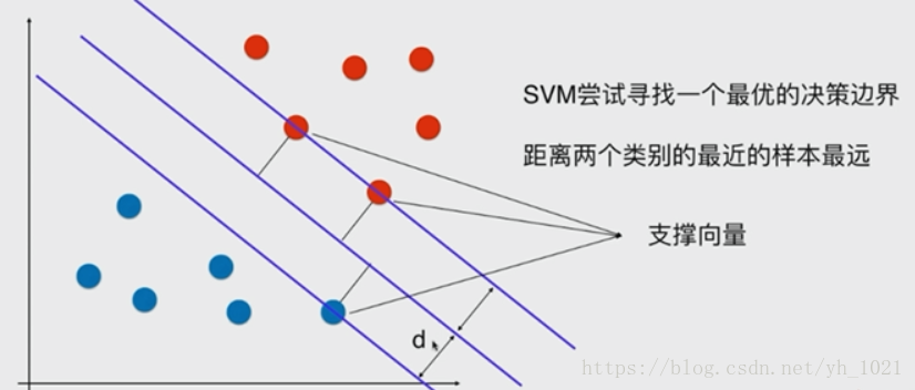
在边界线上的数据点叫做支撑向量,两条边界线之间的距离叫做margin(2*d),中间的线叫做最优决策边界,而svm分类器要做的,就是最大化这个margin。这种方法是解决线性可分问题,叫做Hard Margin SVM,解决线性不可分的问题需要用Soft Margin SVM。
2、数学推导(Hard Margin SVM)
(x,y)到直线Ax+By+C=0的距离为∣Ax+By+C∣A2+B2\frac{\left | Ax+By+C \right |}{\sqrt{A^{2}+B^{2}}}A2+B2∣Ax+By+C∣,拓展到n维空间,到中间直线wTx+b=0w^{T}x+b=0wTx+b=0的距离为∣wT+b∣∥w∥\frac{\left | w^{T}+b \right |}{\left \| w \right \|}∥w∥∣wT+b∣,其中∥w∥=w12+w22+...+wn2\left \| w \right \|=\sqrt{w_{1}^{2}+w_{2}^{2}+...+w_{n}^{2}}∥w∥=w12+w22+...+wn2。
若点到直线的距离>d,则y取1;若将点带入距离公式并去掉绝对值<-d,则y取0>。将d除到左边后可以得到式子:
wTx(i)+b≥1w^{T}x^{\left ( i \right )}+b\geq 1wTx(i)+b≥1,则y取1;wTx(i)+b≤−1w^{T}x^{\left ( i \right )}+b\leq -1wTx(i)+b≤−1,则y取0。
还可以化简为:y(i)(wTx(i)+b)≥1y^{\left ( i \right )}\left ( w^{T}x^{\left ( i \right )}+b \right )\geq 1y(i)(wTx(i)+b)≥1
目标函数为:max∣wT+b∣∥w∥\frac{\left | w^{T}+b \right |}{\left \| w \right \|}∥w∥∣wT+b∣,因为支持向量带入决策边界方程后分子均为1,所以
目标函数:在:y(i)(wTx(i)+b)≥1y^{\left ( i \right )}\left ( w^{T}x^{\left ( i \right )}+b \right )\geq 1y(i)(wTx(i)+b)≥1的条件下max1∥w∥\frac{1}{\left \| w \right \|}∥w∥1,(最小化12∥w∥2\frac{1}{2}\left \|w \right \|^221∥w∥2),这是有条件的最优化问题。
3、Soft Margin和SVM的正则化
为了提高泛化能力和容错能力,在分类时需要不考虑一些极度特殊的点和错误的点。所以就要用到soft margin svm。因为在hard margin svm中,给定的限定条件是必须在>1和<-1的两根直线之外,为了增加容错能力,将两根直线之间的距离稍微小一点(即允许两根线之间有一些点)。需满足:
y(i)(wTx(i)+b)≥1−ξiy^{\left ( i \right )}\left ( w^{T}x^{\left ( i \right )}+b \right )\geq 1-\xi_{i}y(i)(wTx(i)+b)≥1−ξi,(ξi≥0\xi _{i}\geq 0ξi≥0)
为了不使ξ\xiξ无穷大,在目标函数后面增加一项,变成:
min12∥w∥2+∑i=1mCξi\frac{1}{2}\left \| w \right \|^2+\sum_{i=1}^{m}C\xi _{i}21∥w∥2+∑i=1mCξi
这样使得最小化目标函数的同时能有效抑制ξ\xiξ,同时该项也起到了L1正则化的目的,当然L2正则化就是使用的ξ\xiξ的平方。
C的值越小,给予的容错空间越大,当C=0时,就为Hard Margin SVM。
4、sklearn中实现SVM(分类)
因为计算最大间隔涉及距离,所以如果在不同的维度上量纲不同的话,会使得量纲大的那个维度的数占主导地位。所以在进行svm之前也需要做数据的标准化处理。
import numpy as np
import matplotlib.pyplot as plt
from sklearn import datasets
iris=datasets.load_iris()
x=iris.data
y=iris.target
#这里只做二分类问题
x=x[y<2,:2]
y=y[y<2]
plt.scatter(x[y==0,0],x[y==1,1],color='r')
plt.scatter(x[y==1,0],x[y==1,1],color='b')
plt.show()
#对数据进行标准化
from sklearn.preprocessing import StandardScaler
standardscaler=StandardScaler()
standardscaler.fit(x)
x_standard=standardscaler.transform(x)
#加载线性SVM,进行分类工作
##SVC默认采用ovr,多分类时可以改成ovo;默认使用L2方式,也可以使用L1正则化
from sklearn.svm import LinearSVC
svc=LinearSVC(C=1e11) #C取值越小,容错空间越大
svc.fit(x_standard,y)
#画出决策边界以及两条边界线
def plot_svc(axis):
w0=svc.coef_[0]
b=svc.intercept_[0]
#w0*x0+w1*x1+b=0 x1=-w0/w1*x0-b/w1
plot_x=np.linspace(axis[0],axis[1],200)
plot_y=-w0[0]/w0[1]*plot_x-b/w0[1]
#画出svm的上下边界,w0*x0+w1*x1+b=1 ,x1=-w0/w1*x0-b/w1+1/w1
up_y=-w0[0]/w0[1]*plot_x-b/w0[1]+1/w0[1]
down_y=-w0[0]/w0[1]*plot_x-b/w0[1]-1/w0[1]
plt.plot(plot_x,plot_y,color='black')
#将上下边界的y轴范围确定在图的范围之内
up_index=(up_y>=axis[2])&(up_y<=axis[3])
down_index=(down_y>=axis[2])&(down_y<=axis[3])
plt.plot(plot_x[up_index],up_y[up_index],color="r")
plt.plot(plot_x[down_index],down_y[down_index],color="r")
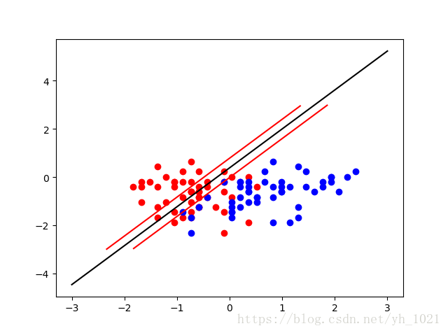
plot_svc(axis=[-3,3,-3,3])
#必须用标准化后的数据进行画图
plt.scatter(x_standard[y==0,0],x_standard[y==1,1],color='r')
plt.scatter(x_standard[y==1,0],x_standard[y==1,1],color='b')
plt.show()
当C的值取的很大(=1e11)时,容错区间较小
当C的值较小(C=0.1)时,容错空间较大
5、非线性SVM
(1)使用多项式特征的SVM
- 用PolynomialFeatures生成多项式特征
- 用StandardScaler进行数据归一化
- 再利用LinearSVC线性SVM模型
import numpy as np
import matplotlib.pyplot as plt
from sklearn import datasets
#用datasets自己生成数据集
x,y=datasets.make_moons(noise=0.1,random_state=666)   #增加数据标准差,加入噪音
plt.scatter(x[y==0,0],x[y==0,1],color='r')
plt.scatter(x[y==1,0],x[y==1,1],color='b')
plt.show()

#使用多项式特征的SVM
from sklearn.preprocessing import PolynomialFeatures,StandardScaler
from sklearn.svm import  LinearSVC
from sklearn.pipeline import Pipeline

def polynomialsvc(degree,C=1.0):
    return Pipeline([
        ("poly",PolynomialFeatures(degree=degree)),
        ("std_scaler",StandardScaler()),
        ("linear_svc",LinearSVC(C=C))
    ])
poly_svc=polynomialsvc(degree=3)
poly_svc.fit(x,y)
print(poly_svc.fit(x,y))

def plot_decision_boundary(model, axis):
    x0, x1 = np.meshgrid(
        np.linspace(axis[0], axis[1], int((axis[1] - axis[0]) * 100)).reshape(-1, 1),
        np.linspace(axis[2], axis[3], int((axis[3] - axis[2]) * 100)).reshape(-1, 1)
    )
    X_new = np.c_[x0.ravel(), x1.ravel()]

    y_predict = model.predict(X_new)
    zz = y_predict.reshape(x0.shape)

    from matplotlib.colors import  ListedColormap
    custom_map=ListedColormap(['#EF9A9A','#FFF59D','#90CAF9'])
    plt.contourf(x0,x1,zz,linewidth=5,cmap=custom_map)

plot_decision_boundary(poly_svc,axis=[-1.5,2.5,-1,2])
plt.scatter(x[y==0,0],x[y==0,1],color='r')
plt.scatter(x[y==1,0],x[y==1,1],color='b')
plt.show()
(2)使用多项式核函数的SVM
- 对数据进行归一化
- 利用核函数SVC(kernel=‘poly’, degree=degree, C=C) (自动多项式化)
from sklearn.svm import SVC
def PolynominalKernelSVC(degree,C=1.0):
    return Pipeline([
        ("sed_scaler",StandardScaler()),
        ("kernel_svc",SVC(kernel='poly'))
    ])
poly_kernel_svc=PolynominalKernelSVC(degree=3)
poly_kernel_svc.fit(x,y)
def plot_decision_boundary(model, axis):
    x0, x1 = np.meshgrid(
        np.linspace(axis[0], axis[1], int((axis[1] - axis[0]) * 100)).reshape(-1, 1),
        np.linspace(axis[2], axis[3], int((axis[3] - axis[2]) * 100)).reshape(-1, 1)
    )
    X_new = np.c_[x0.ravel(), x1.ravel()]
    y_predict = model.predict(X_new)
    zz = y_predict.reshape(x0.shape)
    from matplotlib.colors import  ListedColormap
    custom_map=ListedColormap(['#EF9A9A','#FFF59D','#90CAF9'])
    plt.contourf(x0,x1,zz,linewidth=5,cmap=custom_map)
plot_decision_boundary(poly_kernel_svc,axis=[-1.5,2.5,-1,2])
plt.scatter(x[y==0,0],x[y==0,1],color='r')
plt.scatter(x[y==1,0],x[y==1,1],color='b')
plt.show()
多项式核函数:K(x,y)=(x⋅y+c)dK\left ( x,y \right )=\left ( x\cdot y+c \right )^{d}K(x,y)=(x⋅y+c)d
线性核函数:K(x,y)=x⋅yK\left ( x,y \right )=x\cdot yK(x,y)=x⋅y
高斯核函数:K(x,y)=e−γ∥x−y∥2K\left ( x,y \right )=e^{-\gamma\left \| x-y \right \|^{2} }K(x,y)=e−γ∥x−y∥2
(3)高斯核函数以及sklearn实现
K(x,y)=e−γ∥x−y∥2K\left ( x,y \right )=e^{-\gamma\left \| x-y \right \|^{2} }K(x,y)=e−γ∥x−y∥2
在高斯函数中,gamma越大,高斯分布越窄,gamma越小,高斯分布越宽
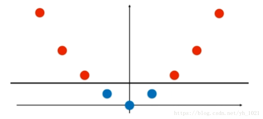
依靠升维使得原本线性不可分的数据线性可分。
假设有两类数据,分部在x轴上,如图所示这组数据是线性不可分的,即无法用直线将红和蓝分开。
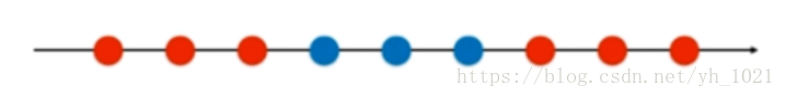
但是将数据升维,增加一个y轴的维度(=x2x^{2}x2),数据就变得线性可分了。
将高斯核函数K(x,y)=e−γ∥x−y∥2K\left ( x,y \right )=e^{-\gamma\left \| x-y \right \|^{2} }K(x,y)=e−γ∥x−y∥2中的y固定为l1和l2,把一维的数据坐标x变成二维的坐标(e−γ∥x−l1∥2,e−γ∥x−l2∥2)\left ( e^{-\gamma \left \| x-l_{1} \right \|^{2}},e^{-\gamma \left \| x-l_{2} \right \|^{2}} \right )(e−γ∥x−l1∥2,e−γ∥x−l2∥2)

import numpy as np
import matplotlib.pyplot as plt
from sklearn import datasets
#用datasets自己生成数据集
x,y=datasets.make_moons(noise=0.1,random_state=666)   #增加数据标准差,加入噪音
plt.scatter(x[y==0,0],x[y==0,1],color='r')
plt.scatter(x[y==1,0],x[y==1,1],color='b')
plt.show()

#用sklearn中的高斯核
from sklearn.preprocessing import StandardScaler
from sklearn.pipeline import Pipeline
from sklearn.svm import SVC

def RBFkernelSVC(gamma=1.0):
    return Pipeline([
        ("std_scaler",StandardScaler()),
        ("svc",SVC(kernel="rbf",gamma=gamma))
    ])
svc=RBFkernelSVC(gamma=1.0)
svc.fit(x,y)

def plot_decision_boundary(model, axis):
    x0, x1 = np.meshgrid(
        np.linspace(axis[0], axis[1], int((axis[1] - axis[0]) * 100)).reshape(-1, 1),
        np.linspace(axis[2], axis[3], int((axis[3] - axis[2]) * 100)).reshape(-1, 1)
    )
    X_new = np.c_[x0.ravel(), x1.ravel()]

    y_predict = model.predict(X_new)
    zz = y_predict.reshape(x0.shape)

    from matplotlib.colors import  ListedColormap
    custom_map=ListedColormap(['#EF9A9A','#FFF59D','#90CAF9'])
    plt.contourf(x0,x1,zz,linewidth=5,cmap=custom_map)

plot_decision_boundary(svc,axis=[-1.5,2.5,-1,2])
plt.scatter(x[y==0,0],x[y==0,1],color='r')
plt.scatter(x[y==1,0],x[y==1,1],color='b')
plt.show()
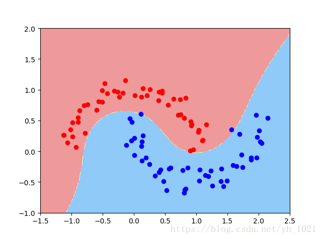
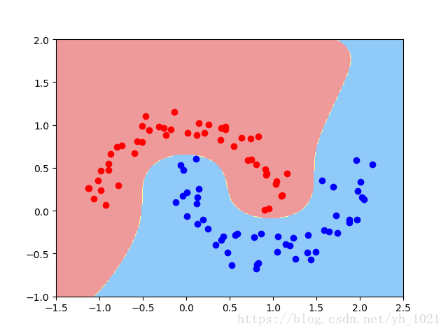
利用rbf内核,gamma取值为1的时候画出决策边界
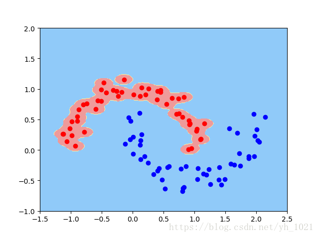
当gamma=100时(因为gamma越大,高斯分布的范围越窄)
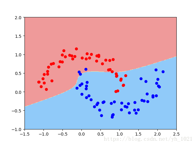
当gamma=0.1时
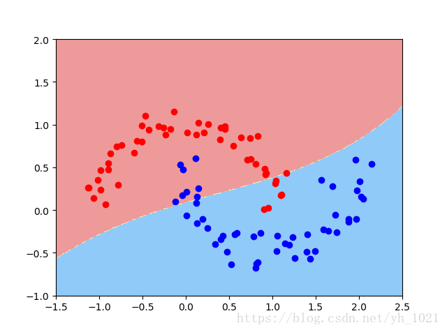
可以看出,当gamma值越大,高斯分布的中心范围越窄,也就是以每一个点为中心周边围绕的区域变小,当然这样的gamma值使得模型过拟合了(泛化能力低);当gamma值很小,高斯分布的中心范围就会变得很大,每一个点的周边范围也会变得很大,如上图所示分界线近似于一条直线,这也就变成了欠拟合。
从另一个角度来说,gamma影响着模型的复杂度,gamma值越小,模型复杂度越小(欠拟合),gamma值越大,模型负责度越大(过拟合)。
6、用SVM实现回归问题
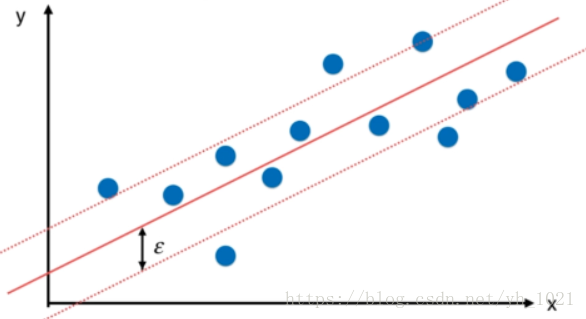
在分类任务中,我们利用了决策边界直线进行分割,并且得到了使得margin区域最大时的上下边界,在这个边界中不允许有数据点存在。而在回归问题中,我们也可以使用上下边界的概念,在得到拟合曲线之后,我们定义距离拟合曲线margin(ϵ\epsilonϵ)的两条直线为上下边界,与分类问题相反,在上下边界中包含的数据点的个数越多越好。
from sklearn import datasets

boston=datasets.load_boston()
x=boston.data
y=boston.target

from sklearn.model_selection import train_test_split
x_train,x_test,y_train,y_test=train_test_split(x,y,random_state=666)

#使用svm中的回归函数
from sklearn.svm import LinearSVR
from sklearn.svm import SVR
from sklearn.preprocessing import StandardScaler
from sklearn.pipeline import Pipeline

def standardLinearSVR(epsilon=0.1):
    return Pipeline([
        ("std_scaler",StandardScaler()),
        ("linearSVR",LinearSVR(epsilon=epsilon))
    ])
svr=standardLinearSVR()
svr.fit(x_train,y_train)
print(svr.score(x_test,y_test))
可以使用LinearSVR也可以使用SVR,使用LinearSVR时可以改变epsilon的值,C的值;使用SVR时可以改变的超参数有核函数,可以使用高斯核,可以改变gamma的值等。可以通过改变各种超参数,或者使用交叉验证的方式,来提高精确度。


 1万+
1万+

 被折叠的 条评论
为什么被折叠?
被折叠的 条评论
为什么被折叠?
 到【灌水乐园】发言


