Machine Learning From Scratch: Logistic Regression

Ref: 

Introduction

After having discussed linear regression in the first part of this series, it’s time to take a look at another building block of more advanced machine learning algorithms: logistic regression. Logistic regression, despite its name, is most widely used for binary classification. In binary classification, you are trying to predict whether an observation belongs either to class 0 or class 1. For instance, one could try to predict whether visitors of a website are going to click on an ad or not.

Preparation

In order to start building logistic regression, we first need to generate some dummy data. To create data from two different classes, we will create two input features, X1 and X2, along with our response variable Y. We’ll draw X1 and X2 from a Gaussian distribution with different means to make them clearly separable.

X1_1 = pd.Series(np.random.randn(5))
X1_2 = pd.Series(np.random.randn(5)+4)
X1 = pd.concat([X1_1, X1_2]).reset_index(drop=True)
X2 = pd.Series(np.random.randn(10))
Y = pd.Series([0,0,0,0,0,1,1,1,1,1])

data = pd.concat([X1, X2, Y], axis=1)
data.columns= ["X1", "X2", "Y"]

Since visualizations are always nice, let’s take a look at our data:

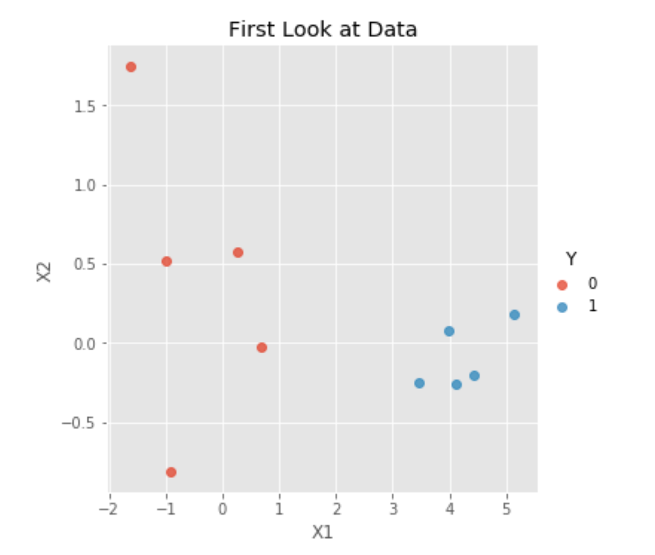
As we can see, our two classes, Y=0 and Y=1, are clearly separable. Thus, fitting a logistic regression might be a good idea. Unfortunately, using a linear regression in this case would not be a very good idea because a linear regression’s outputs are not between zero and one, making it extremely difficult to interpret them as probabilities of Y=0 or Y=1.

Therefore, instead of just sticking to a linear regression with two input features and using Y =beta0 + beta1*X1 + beta2*X2, we are going to transform our linear regression equation using the sigmoid function.

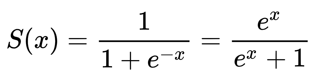
The sigmoid function maps real values to values between zero and one. This way, we’ll be able to interpret our results as probabilities of a specific training instance belonging to class Y=0 or Y=1. The only thing we need to do is define a cutoff probability that’ll separate our classes. For instance, we could, depending on our projects’ requirements, set Y=0 if P≤0.5 and Y=1 if P>0.5.

All that’s left to do now is replacing the x in the sigmoid formula above with our regression equation:

Let’s define a function for that:

def sigmoid(beta0, beta1, beta2, X1, X2):
    """
    Input:
    This function takes the beta parameters beta0, beta1, and beta2,
    as well as X1 and X2 as inputs
    
    Output:
    After having transformed the inputs into a real value between 0
    and 1, the function will return said value that can be interpreted
    as a probability
    """
    prepared = beta0 + beta1*X1 + beta2*X2
    prediction = 1/(1 + np.exp(-prepared))
    return prediction

Gradient Descent

We are going to use stochastic gradient descent to find our optimal parameters. In stochastic gradient descent, as opposed to batch gradient descent, we are only going to use a single observation to update our parameters. Apart from that, the process is basically the same:

1. Initialize the coefficients with zero or small random values
2. Evaluate the cost of these parameters by plugging them into a cost function
3. Calculate the derivative of the cost function
4. Update the parameters scaled by a learning rate/step size

To get a better understanding of this rough outline of gradient descent, let’s look at the Python code.

The first step of gradient descent consists of initializing the parameters with zero or small random values. In our case, we have to initialize beta0, beta1, and beta2:

#let's assign 0 to our betas to initialize them
beta0 = 0.
beta1 = 0.
beta2 = 0.

Now that we have initialized our betas, we can actually use the sigmoid function we defined earlier and understand what it does. By inputting our first training observation, we get the following result:

#selecting our first training observation
X1, X2, Y = list(data.iloc[0,:])

#making our first prediction
first_prediction = sigmoid(beta0, beta1, beta2, X1, X2)
print("Our first prediction is {}".format(first_prediction))
#Output: Our first prediction is 0.5

What does our output mean? The sigmoid function returns a probability. In our case, we haven’t defined a cutoff probability and our betas are all zeros. Thus, the output probabilities of the first training observation belonging to class 1 or 0 are equal. To get better predictions, we’re going to use stochastic gradient descent. To do so, we’re going to have to update our parameters:

def update_coefficients(beta0, beta1, beta2, X1, X2, Y, prediction):
    """
    This function takes the training instance as well as the betas
    and the previously calculated prediction to update the coefficients
    """
    alpha = 0.3
    bias_of_intercept = 1.0
    beta0 = beta0 + alpha*(Y-prediction)*prediction*(1-prediction)*bias_of_intercept
    beta1 = beta1 + alpha*(Y-prediction)*prediction*(1-prediction)*X1
    beta2 = beta2 + alpha*(Y-prediction)*prediction*(1-prediction)*X2
    
    return beta0, beta1, beta2
  
beta0, beta1, beta2 = update_coefficients(beta0, beta1, beta2, X1, X2, Y, first_prediction)
print("Our updated parameters are:\nbeta0: {}\nbeta1: {}\nbeta2: {}".format(beta0, beta1, beta2))
#Output:
#Our updated parameters are:
#beta0: -0.0375
#beta1: -0.020980870585683948
#beta2: -0.03909196554528134

Making Predictions

Functions make our life easier, however, we would still have to repeat this process manually for each of our observations. That doesn’t sound very fun, does it?

Since we’ve defined a few handy functions, we can just put all of them together and loop through our training observations. Note that this works fine with our small dataset, however, it would very likely be a bottleneck when using larger datasets.

def putting_it_together(epochs=1, learning_rate=0.3, cutoff=0.5):
    """
    This function performs a stochastic gradient descent
    and returns the final coefficients
    """
    beta0 = 0.
    beta1 = 0.
    beta2 = 0.
    bias_of_intercept = 1.0
    alpha = learning_rate
    

    for i in range(1,epochs+1):
        
        correct_predictions = 0
        print('\nThis is epoch number {}:\n'.format(i), '-'*60)
        
        for n in range(len(data.X1)):

            X1 = data.iloc[n,0]
            X2 = data.iloc[n,1]
            Y = data.iloc[n,2]

            prediction = sigmoid(beta0, beta1, beta2, X1, X2)

            beta0, beta1, beta2 = update_coefficients(beta0, beta1, beta2, X1, X2, Y, prediction)
            
            if prediction < cutoff:
                class_ = 0
            else:
                class_ = 1
                
            if class_ == Y:
                correct_predictions+=1
            else:
                continue

            print('(Instance Number {}) Beta0: {:.3f}, Beta1: {:.3f}, Beta2: {:.3f}, prediction: {}, class: {}, actual class: {}'.format(n+1, beta0, beta1, beta2, prediction, class_, Y))
        
        accuracy = (correct_predictions/len(data.X1))*100
        print('\nAccuracy of this epoch: {}%\n'.format(accuracy), '-'*60)
    return beta0, beta1, beta2

Let’s walk through this: the parameters we have to define for our function are the number of epochs, the learning rate, and the cutoff probability. An epoch defines using stochastic gradient descent on each of our training observations once. The learning rate defines by how much we’d like to scale our step size in gradient descent. The bigger, the larger the step size but also the greater the risk of overshooting the minimum. Lastly, the cutoff probability helps us use the outputs of the sigmoid function to make class membership predictions.

First, we initialize the parameters to zero like we did earlier. Inside of the function, there are two for-loops. The first one is iterating over the number of epochs defined by us. Within this for-loop, there’s another for-loop iterating over each of our training observations.

When running this for-loop, we select each training observation’s X1, X2, and Y values one by one to perform our computations. First, we put our parameters into the sigmoid function and get a probability as a result. Then, we update our coefficients and use the cutoff probability to determine whether that specific training observation is class 1 or class 0. Simultaneously, we’re counting all correct predictions by comparing our predictions with the actual Y values for each training observation. The accuracy is then calculated by dividing the number of correct predictions by the total number of predictions. Expressed a little more formally we get:

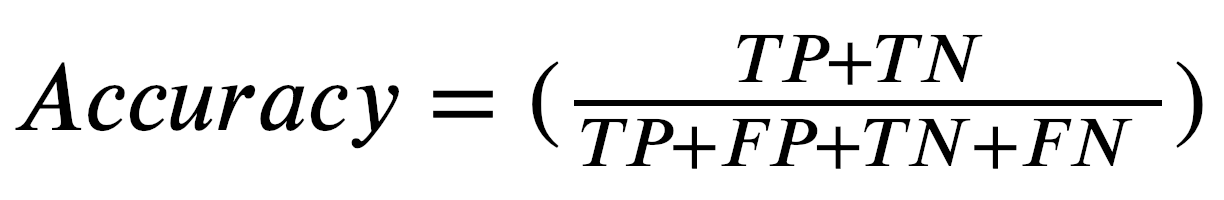
where TP = True Positive, TN = True Negative, FP = False Positive, FN = False Negative

Now comes the fun part: running our function. In this example, I’ve set the cutoff probability to 0.51. In Python, we do the following:

putting_it_together(cutoff = 0.51)

#Output:
#This is epoch number 1:
# ------------------------------------------------------------
#(Instance Number 1) Beta0: -0.037, Beta1: -0.021, Beta2: -0.039, prediction: 0.5, class: 0, actual class: 0
#(Instance Number 2) Beta0: -0.074, Beta1: -0.010, Beta2: -0.035, prediction: 0.49318256187851595, class: 0, actual class: 0
#(Instance Number 3) Beta0: -0.110, Beta1: 0.030, Beta2: -0.061, prediction: 0.4777504730569901, class: 0, actual class: 0
#(Instance Number 4) Beta0: -0.144, Beta1: 0.069, Beta2: -0.078, prediction: 0.45645333162008134, class: 0, actual class: 0
#(Instance Number 5) Beta0: -0.181, Beta1: 0.104, Beta2: -0.008, prediction: 0.48480217726825375, class: 0, actual class: 0
#(Instance Number 6) Beta0: -0.148, Beta1: 0.239, Beta2: 0.003, prediction: 0.5623015703558849, class: 1, actual class: 1
#(Instance Number 7) Beta0: -0.130, Beta1: 0.317, Beta2: 0.018, prediction: 0.709114917067449, class: 1, actual class: 1
#(Instance Number 8) Beta0: -0.121, Beta1: 0.361, Beta2: 0.006, prediction: 0.8095023471228494, class: 1, actual class: 1
#(Instance Number 9) Beta0: -0.099, Beta1: 0.410, Beta2: 0.063, prediction: 0.661298222653969, class: 1, actual class: 1
#(Instance Number 10) Beta0: -0.094, Beta1: 0.433, Beta2: 0.070, prediction: 0.8608443171411484, class: 1, actual class: 1

#Accuracy of this epoch: 100.0%
# ------------------------------------------------------------

Thanks to our previously defined function, we get a very clean and informative output. For each training observation, we see how our betas are getting updated as well as the class prediction. Most importantly though, we can compare our predicted class membership with the actual class membership. Within just one epoch, we’ve achieved 100% accuracy!

As always, if you have any feedback or found mistakes, please don’t hesitate to reach out to me.

The complete notebook can be found on my GitHub: https://github.com/lksfr/MachineLearningFromScratch