学习opencv: 使用边缘信息提升全局阈值分割的性能

Using Edges to Improve Global Thresholding

---

突然发现可以从本地导入markdown文档，哈哈哈哈哈

---

使用全局阈值分割图像的一个基本条件是前景和背景的直方图波峰之间有足够的空隙，这样将阈值设置在空隙之间就可以将前景和背景分开。一个***好的***直方图，也就是适合使用全局阈值分割的直方图往往具有如下特征：

• tall
• narrow
• symmetric
• separated by deep valleys

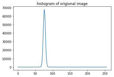
然而有时候人眼看起来前景和背景对比度很高，很容易用全局阈值分割的图像却不容易自适应地找到阈值，因为前景或者背景内容太多，导致另一方在灰度直方图中的贡献被淹没了，本实验要解决的就是这个问题。

解决这个问题的中心思想是只对前景和背景相邻的地方统计直方图。而找到相邻的地方往往可以通过magnitude of gradient of image 或者Laplacian operator得到。

主要的步骤如下：

1. 计算图像‘magnitude of gradient’或者‘absolute value of the Laplacian’
2. 确定一个阈值T
3. 使用2确定的阈值T对第1步中的图像做个二值化，得到的结果作为下一步统计直方图的mask
4. 上一步得到的mask对原始图像计算灰度直方图
5. 对4中得到的直方图求自适应的阈值
6. 使用5中得到的阈值进行阈值分割即可

通过上面的介绍可以发现***适合使用该方法分割的图像应该具有如下特点***：

• 图像本身边缘就相对比较清晰，通过一定方法可以大致找到
• 适合前景和背景面积相对较悬殊的情况

import os 
import cv2
import numpy as np
import matplotlib.pyplot as plt

os.chdir('C:/Users/new_xuyangcao/Desktop/ImageProcessing/test')

#load image and transform to gray
img = cv2.imread('septagon.tif')
gray = cv2.cvtColor(img, cv2.COLOR_BGR2GRAY)
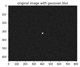
gray = cv2.GaussianBlur(gray, (5, 5), 0)
plt.figure(), plt.imshow(gray, cmap = 'gray')
plt.title('original image with gaussian blur')

#histogram of the origional image
hist = cv2.calcHist([gray], [0], None, [256], [0, 256])
plt.figure(), plt.plot(hist)
plt.title('histogram of origional image')

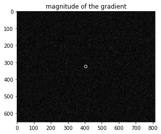
'''step 1: The magnitude of the gradient image'''
gray1 = np.double(gray)
x = cv2.Sobel(gray1, -1, 1, 0)
y = cv2.Sobel(gray1, -1, 0, 1)
grad = (np.sqrt(x**2 + y**2))
plt.figure(), plt.imshow(grad, cmap = 'gray')
plt.title('magnitude of the gradient')

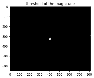
'''step 2: Specify a threshold T and threshold the image from step 1,
           then using it as a mask image '''
_, mask_bw = cv2.threshold(np.uint8(grad), np.int(np.max(grad))*0.2, 255, cv2.THRESH_BINARY)
plt.figure(), plt.imshow(mask_bw, cmap = 'gray')
plt.title('threshold of the magnitude')

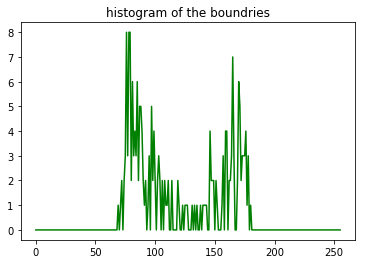
'''step 3: Count a theshold of the image of step2 '''
hist = cv2.calcHist([gray], [0], mask_bw, [256], [0, 256])
hist[0] = 0
plt.figure(), plt.plot(hist, color = 'g')
plt.title('histogram of the boundries')

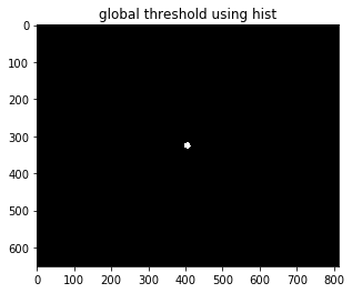
'''step 4: Using the threshold from step 3 to threshod'''
_, bw = cv2.threshold(gray, 125, 255, cv2.THRESH_BINARY)
plt.figure(), plt.imshow(bw, cmap = 'gray')
plt.title('global threshold using hist')

plt.show()

参考资料：Rafael C. Gonzalez, et al. Digital Image Processing Third Edition[M]