用600样本训练的XGBoost模型，可以达到 R²: 0.9429

用600样本，看XGBoost能够做到什么程度：

import numpy as np
import pandas as pd
from sklearn.datasets import make_regression
from sklearn.model_selection import train_test_split, GridSearchCV
from sklearn.metrics import mean_squared_error, r2_score
import xgboost as xgb
import matplotlib.pyplot as plt


# 1. 生成模拟数据（600样本，10特征）
X, y = make_regression(n_samples=600, n_features=10, noise=0.1, random_state=42)
df = pd.DataFrame(X, columns=[f'feat_{i}' for i in range(10)])
df['target'] = y

# 2. 数据预处理
X = df.drop('target', axis=1)
y = df['target']

# 划分训练集和测试集（80%训练，20%测试）
X_train, X_test, y_train, y_test = train_test_split(
    X, y, test_size=0.2, random_state=42)

# 特征标准化（对回归问题通常需要）
from sklearn.preprocessing import StandardScaler
scaler = StandardScaler()
X_train_scaled = scaler.fit_transform(X_train)
X_test_scaled = scaler.transform(X_test)

# 3. 基础模型构建（防止过拟合参数）
base_params = {
    'objective': 'reg:squarederror',
    'eval_metric': 'rmse',
    'booster': 'gbtree',
    'n_jobs': -1,
    'random_state': 42,
    'max_depth': 3,          # 限制树深度
    'learning_rate': 0.1,    # 较低学习率
    'subsample': 0.8,        # 行采样
    'colsample_bytree': 0.7, # 特征采样
    'reg_alpha': 0.5,        # L1正则化
    'reg_lambda': 1.0        # L2正则化
}

# 4. 网格搜索调参（优化关键参数）
param_grid = {
    'n_estimators': [100, 200, 300],
    'max_depth': [3, 4],
    'learning_rate': [0.05, 0.1],
    'min_child_weight': [5, 10]  # 控制叶子节点样本权重
}

# 使用5折交叉验证
grid_search = GridSearchCV(
    estimator=xgb.XGBRegressor(**base_params),
    param_grid=param_grid,
    scoring='neg_mean_squared_error',
    cv=5,
    n_jobs=-1,
    verbose=1
)

grid_search.fit(X_train_scaled, y_train)

# 输出最佳参数
print(f"Best parameters: {grid_search.best_params_}")
print(f"Best CV RMSE: {-grid_search.best_score_:.4f}")

# 5. 最终模型训练
best_model = grid_search.best_estimator_
eval_set = [(X_train_scaled, y_train), (X_test_scaled, y_test)]

best_model.fit(
    X_train_scaled, 
    y_train,
    eval_set=eval_set,
    verbose=False)

# 6. 模型评估
y_pred = best_model.predict(X_test_scaled)

# 计算RMSE（手动计算平方根）
mse = mean_squared_error(y_test, y_pred)
rmse = np.sqrt(mse)
r2 = r2_score(y_test, y_pred)

print(f"Test RMSE: {rmse:.4f}")
print(f"Test R²: {r2:.4f}")

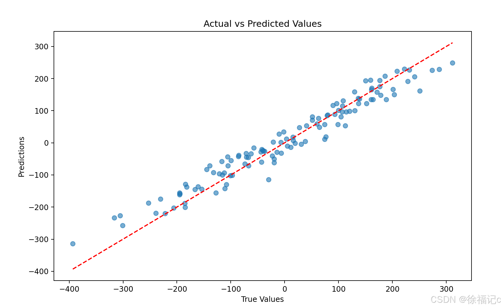
# 7. 可视化预测结果
plt.figure(figsize=(10, 6))
plt.scatter(y_test, y_pred, alpha=0.6)
plt.plot([y_test.min(), y_test.max()], [y_test.min(), y_test.max()], 'r--')
plt.xlabel('True Values')
plt.ylabel('Predictions')
plt.title('Actual vs Predicted Values')
plt.show()

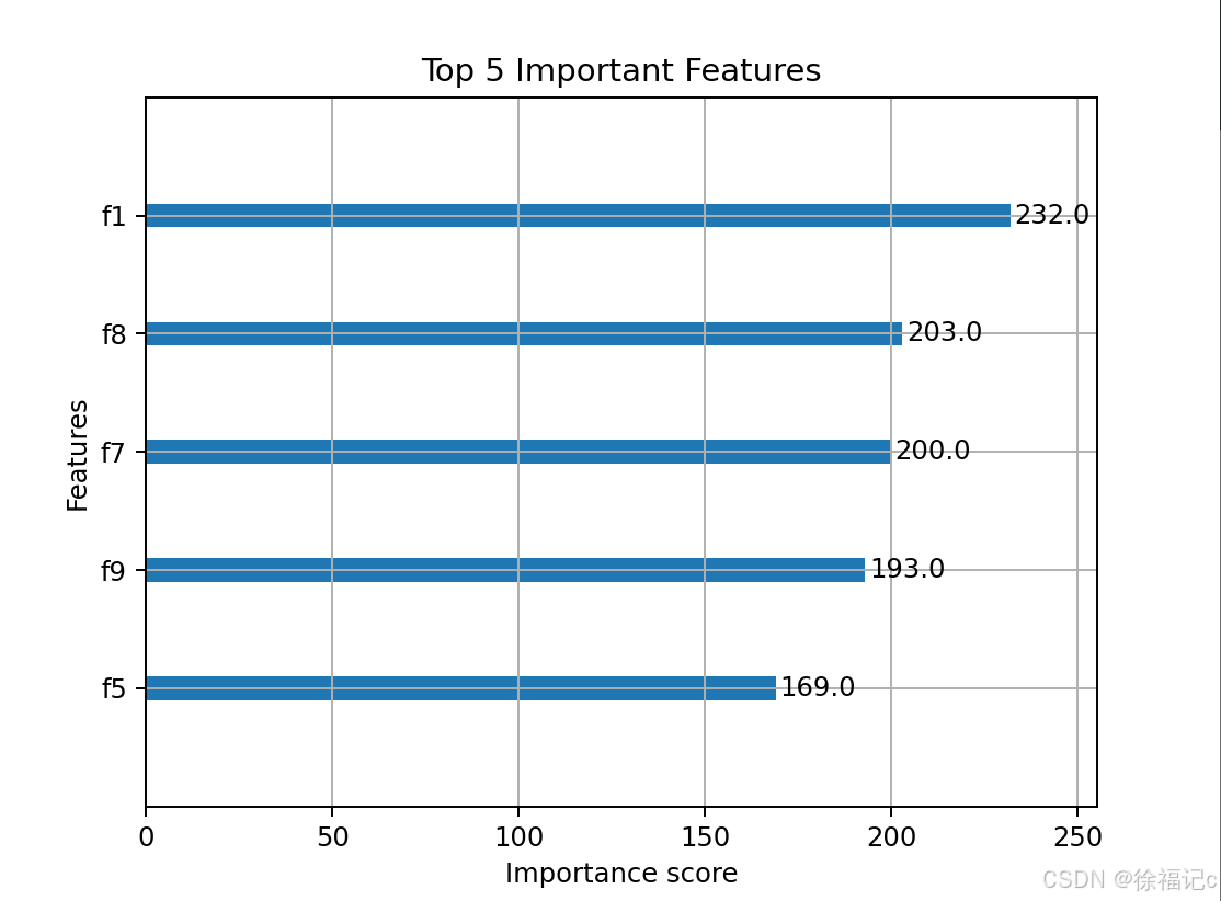
# 8. 特征重要性分析
xgb.plot_importance(best_model, max_num_features=5)
plt.title('Top 5 Important Features')
plt.show()

运行之后：

Fitting 5 folds for each of 24 candidates, totalling 120 fits
Best parameters: {'learning_rate': 0.1, 'max_depth': 3, 'min_child_weight': 5, 'n_estimators': 300}
Best CV RMSE: 1627.6646
Test RMSE: 35.1356
Test R²: 0.9429