Package funModeling: data cleaning, importance variable analysis and model perfomance

(This article was first published on  R - Data Science Heroes Blog, and kindly contributed to  R-bloggers)

Hi there 

This new package –install.packages("funModeling")– tries to cover with simple concepts common tasks in data science. Written like a short tutorial, its focus is on data interpretation and analysis.

Below, you’ll find a copy-paste from the package vignette, (so you can drink a good coffee while you read it… )

---

Introduction

This package covers common aspects in predictive modeling:

1. Data Cleaning
2. Variable importance analysis
3. Assessing model performance

Main purpose of this package is to teach some predictive modeling using a practical toolbox of functions and concepts, to people who is starting in data science, small data and big data. With special focus on results and analysis understanding.

Part 1: Data cleaning

Overview: Quantity of zeros, NA, unique values; as well as the data type may lead to a good or bad model. Here an approach to cover the very first step in data modeling.

## Loading needed libraries
library(funModeling)  
data(heart_disease)  

Checking NA, zeros, data type and unique values

my_data_status=df_status(heart_disease)  

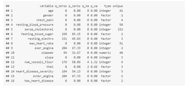
• q_zeros: quantity of zeros (p_zeros: in percentage)
• q_na: quantity of NA (p_na: in percentage)
• type: factor or numeric
• unique: quantity of unique values

Why are these metrics important?

• Zeros: Variables with lots of zeros may be not useful for modeling, and in some cases it may dramatically bias the model.
• NA: Several models automatically exclude rows with NA (random forest, for example). As a result, the final model can be biased due to several missing rows because of only one variable. For example, if the data contains only one out of 100 variables with 90% of NAs, the model will be training with only 10% of original rows.
• Type: Some variables are encoded as numbers, but they are codes or categories, and the models don’t handle them in the same way.
• Unique: Factor/categorical variables with a high number of different values (~30), tend to do overfitting if categories have low representative, (decision tree, for example).

Filtering unwanted cases

Function df_status takes a data frame and returns a the status table to quickly remove unwanted cases.

Removing variables with high number of NA/zeros

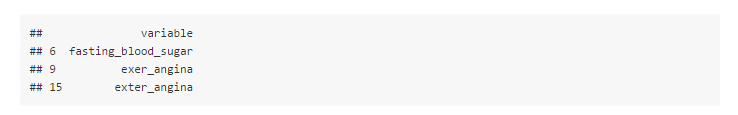
# Removing variables with 60% of zero values
vars_to_remove=subset(my_data_status, my_data_status$p_zeros > 60)  
vars_to_remove["variable"]  

## Keeping all except vars_to_remove 
heart_disease_2=heart_disease[, !(names(heart_disease) %in% vars_to_remove[,"variable"])]

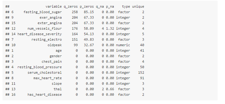
Ordering data by percentage of zeros

my_data_status[order(-my_data_status$p_zeros),]  

Part 2: Variable importance with cross_plot

• Overview:
  • Analysis purpose: To identify if the input variable is a good/bad predictor through visual analysis.
  • General purpose: To explain the decision of including -or not- a variable to a model to a non-analyst person.

Constraint: Target variable must have only 2 values. If it has NAvalues, they will be removed.

Note: Please note there are many ways for selecting best variables to build a model, here is presented one more based on visual analysis.

Example 1: Is gender correlated with heart disease?

cross_gender=cross_plot(heart_disease, str_input="gender", str_target="has_heart_disease")  

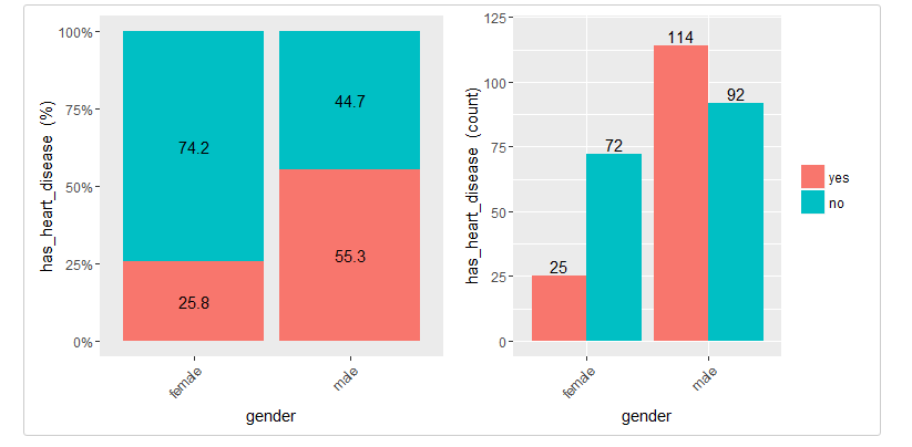
Last two plots have the same data source, showing the distribution of has_heart_disease in terms of gender. The one on the left shows in percentage value, while the one on the right shows in absolute value.

How to extract conclusions from the plots? (Short version)

Gender variable seems to be a good predictor, since the likelihood of having heart disease is different given the female/male groups. it gives an order to the data.

How to extract conclusions from the plots? (Long version)

From 1st plot (%):

1. The likelihood of having heart disease for males is 55.3%, while for females is: 25.8%.
2. The heart disease rate for males doubles the rate for females (55.3 vs 25.8, respectively).

From 2nd plot (count):

1. There are a total of 97 females:

   • 25 of them have heart disease (25/97=25.8%, which is the ratio of 1st plot).
   • the remaining 72 have not heart disease (74.2%)

2. There are a total of 206 males:

   • 114 of them have heart disease (55.3%)
   • the remaining 92 have not heart disease (44.7%)

3. Total cases: Summing the values of four bars: 25+72+114+92=303.

Note: What would it happened if instead of having the rates of 25.8% vs. 55.3% (female vs male), they had been more similar like 30.2% vs. 30.6%). In this case variable gender it would have been much less relevant, since it doesn’t separate thehas_heart_disease event.

Example 2: Crossing with numerical variables

Numerical variables should be binned in order to plot them with an histogram, otherwise the plot is not showing information, as it can be seen here:

Equal frequency binning

There is a function included in the package (inherited from Hmisc package) : equal_freq, which returns the bins/buckets based on the equal frequency criteria. Which is -or tries to- have the same quantity of rows per bin.

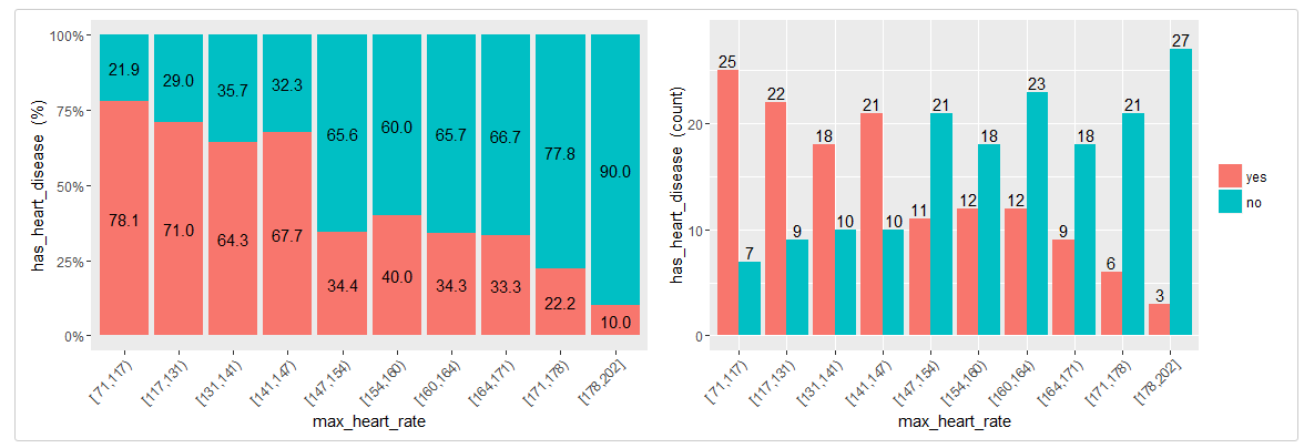
For numerical variables, cross_plot has by default theauto_binning=T, which automtically calls the equal_freqfunction with n_bins=10 (or the closest number).

cross_plot(heart_disease, str_input="max_heart_rate", str_target="has_heart_disease")  

Example 3: Manual binning

If you don’t want the automatic binning, then set theauto_binning=F in cross_plot function.

For example, creating oldpeak_2 based on equal frequency, with 3 buckets.

heart_disease$oldpeak_2=equal_freq(var=heart_disease$oldpeak, n_bins = 3)  
summary(heart_disease$oldpeak_2)  

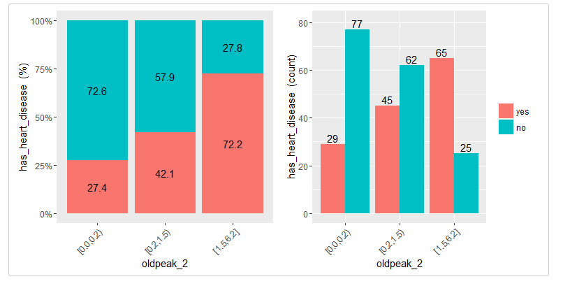
Plotting the binned variable (auto_binning = F):

cross_oldpeak_2=cross_plot(heart_disease, str_input="oldpeak_2", str_target="has_heart_disease", auto_binning = F)  

Conclusion

This new plot based on oldpeak_2 shows clearly how: the likelihood of having heart disease increases as oldpeak_2 increases as well.Again, it gives an order to the data.

Example 3: Noise reducing

Converting variable max_heart_rate into a one of 10 bins:

heart_disease$max_heart_rate_2=equal_freq(var=heart_disease$max_heart_rate, n_bins = 10)  
cross_plot(heart_disease, str_input="max_heart_rate_2", str_target="has_heart_disease")  

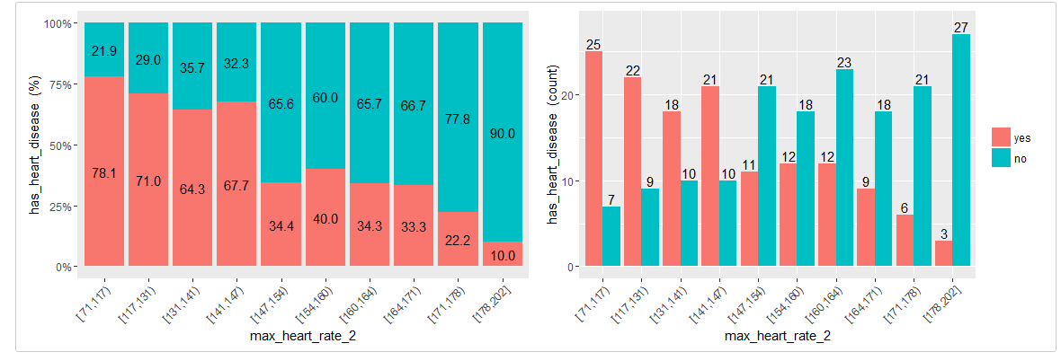
At a first glance, max_heart_rate_2 shows a negative and linear relationship, however there are some buckets which add noise to the relationship. For example, the bucket (141, 146] has a higher heart disease rate than the previous bucket, and it was expected to have a lower. This could be noise in data.

Key note: One way to reduce the noise (at the cost of losing some information), is to split with less bins:

heart_disease$max_heart_rate_3=equal_freq(var=heart_disease$max_heart_rate, n_bins = 5)  
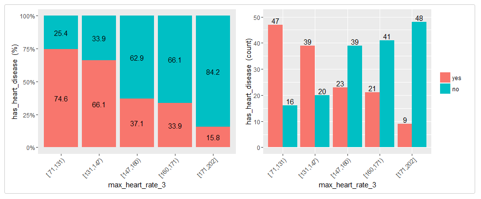
cross_plot(heart_disease, str_input="max_heart_rate_3", str_target="has_heart_disease")  

Conclusion: As it can be seen, now the relationship is much clean and clear. Bucket ‘N’ has a higher rate than ‘N+1′, which implies a negative correlation.

How about saving the cross_plot result into a folder?
Just set the parameter path_out with the folder you want -It creates a new one if it doesn’t exists-.

cross_plot(heart_disease, str_input="max_heart_rate_3", str_target="has_heart_disease", path_out="my_plots")  

It creates the folder my_plots into the working directory.

Example 4: cross_plot on multiple variables

Imagine you want to run cross_plot for several variables at the same time. To achieve this goal you define a list of strings containing all the variables to use as input in the cross_plot, and then, call the function massive_cross_plot.

If you want to analyze these 3 variables:

vars_to_analyze=c("age", "oldpeak", "max_heart_rate")  

massive_cross_plot(data=heart_disease, str_target="has_heart_disease", str_vars=vars_to_analyze)  

Automatically saving all the results into a folder
Same as cross_plot, this function has the path_out parameter.

massive_cross_plot(data=heart_disease, str_target="has_heart_disease", str_vars=vars_to_analyze, path_out="my_plots")  

Final notes:

• Correlation does not imply causation
• cross_plot is good to visualize linear relationships, giving it a hint on non-linear relationships.
• Cleaning the variables help the model to better modelize the data.

Part 3: Assessing model performance

Overview: Once the predictive model is developed with trainingdata, it should be compared with test data (which wasn’t seen by the model before). Here is presented a wrapper for the ROC Curve and AUC (area under ROC) and the KS (Kolmogorov-Smirnov).

Creating the model

## Training and test data. Percentage of training cases default value=80%.
index_sample=get_sample(data=heart_disease, percentage_tr_rows=0.8)

## Generating the samples
data_tr=heart_disease[index_sample,]  
data_ts=heart_disease[-index_sample,]


## Creating the model only with training data
fit_glm=glm(has_heart_disease ~ age + oldpeak, data=data_tr, family = binomial)

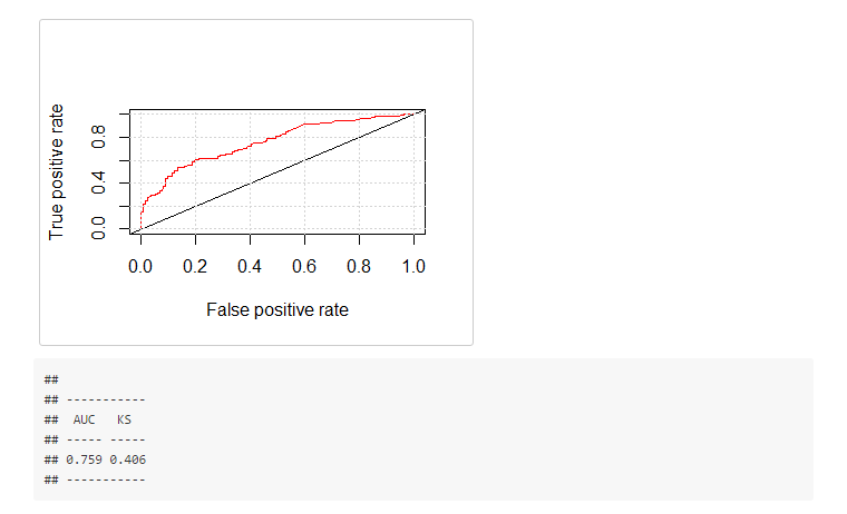
ROC, AUC and KS performance metrics

## Performance metrics for Training Data
model_performance(fit=fit_glm, data = data_tr, target_var = "has_heart_disease")  

## Performance metrics for Test Data
model_performance(fit=fit_glm, data = data_ts, target_var = "has_heart_disease")  

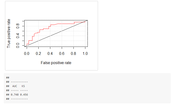
Key notes

• The higher the KS and AUC, the better the performance is.
  • KS range: from 0 to 1.
  • AUC range: from 0.5 to 1.
• Performance metrics should be similar between training and test set.

Final comments

• KS and AUC focus on similar aspects: How well the model distinguishes the class to predict.
• ROC and AUC article: link

---

End of vignette, some links…

Github.
Sneak peek into the  funModeling “black-box”  (either for learning or to contribute -code not complex and commented):