PyTorch基础知识学习记录

1、安装

1. 安装anaconda，已经提前安装过
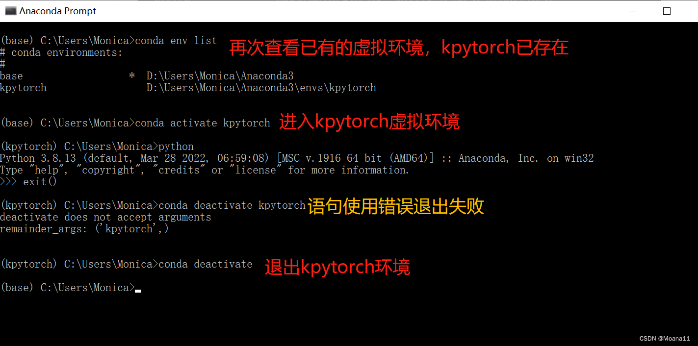
2. 创建虚拟环境(第一次)

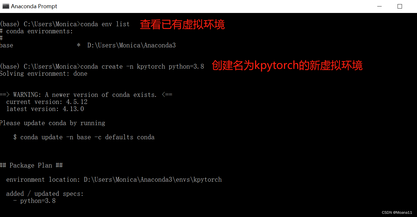
3. conda换源
   Windows系统：
   TUNA 提供了 Anaconda 仓库与第三方源的镜像，各系统都可以通过修改用户目录下的 .condarc 文件。Windows 用户无法直接创建名为 .condarc 的文件，可先执行conda config --set show_channel_urls yes生成该文件之后再修改。

完成这一步后，我们需要修改C:\Users\User_name.condarc这个文件，打开后将文件里原始内容删除，将下面的内容复制进去并保存。

channels:
  - defaults
show_channel_urls: true
default_channels:
  - https://mirrors.tuna.tsinghua.edu.cn/anaconda/pkgs/main
  - https://mirrors.tuna.tsinghua.edu.cn/anaconda/pkgs/r
  - https://mirrors.tuna.tsinghua.edu.cn/anaconda/pkgs/msys2
custom_channels:
  conda-forge: https://mirrors.tuna.tsinghua.edu.cn/anaconda/cloud
  msys2: https://mirrors.tuna.tsinghua.edu.cn/anaconda/cloud
  bioconda: https://mirrors.tuna.tsinghua.edu.cn/anaconda/cloud
  menpo: https://mirrors.tuna.tsinghua.edu.cn/anaconda/cloud
  pytorch: https://mirrors.tuna.tsinghua.edu.cn/anaconda/cloud
  simpleitk: https://mirrors.tuna.tsinghua.edu.cn/anaconda/cloud

这一步完成后，我们需要打开Anaconda Prompt 运行 conda clean -i 清除索引缓存，保证用的是镜像站提供的索引。

**4. 查看显卡驱动发现只能用cuda8.0版本

1. PyTorch官网找到相应版本，安装成功**

# CUDA 8.0
conda install pytorch==1.0.0 torchvision==0.2.1 cuda80 -c pytorch

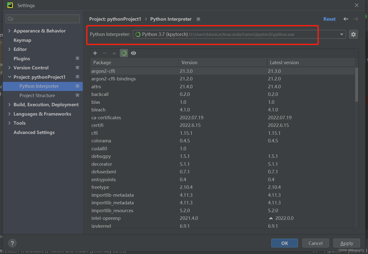
6. 配置pycharm环境（因为已经安装过pycharm，就配置了下环境)

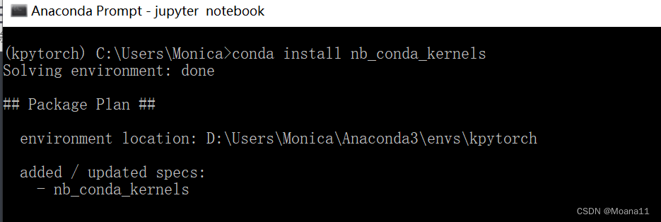
7. PyTorch部署到jupyter中
参考链接：

https://blog.youkuaiyun.com/weixin_45527999/article/details/124574230

在anaconda prompt中进入kpytorch环境

conda install nb_conda_kernels

2、PyTorch基础知识

2.1张量

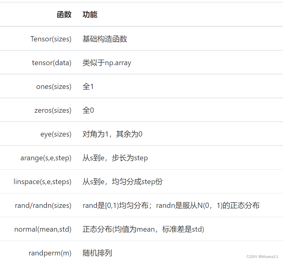
2.1.1创建张量

#创建随机矩阵
import torch
x = torch.rand(2,3)
print('创建随机矩阵：\n')
print(x)
y = torch.tensor([[1,3.92,5,7.0],[2,4.259,6,8],[0,5,9.6,2]],dtype=torch.float)
print('\n直接构建张量:\n')
print(y)

结果：

创建随机矩阵：

tensor([[0.9012, 0.6873, 0.3820],
        [0.3951, 0.9004, 0.1177]])

直接构建张量:

tensor([[1.0000, 3.9200, 5.0000, 7.0000],
        [2.0000, 4.2590, 6.0000, 8.0000],
        [0.0000, 5.0000, 9.6000, 2.0000]])

#构建全0全1 矩阵
import torch
x = torch.zeros(3,4,dtype=torch.long)
print('全0矩阵：\n',x)

y = torch.ones(3,2,dtype=torch.float)
print('全1矩阵：\n',y)
z = torch.eye(4,4,dtype=torch.int)
print('对角矩阵：\n',z)

x = x.new_ones(4,3,dtype=torch.double)  #这个new_ones()没太懂
# 创建一个新的全1矩阵tensor，返回的tensor默认具有相同的torch.dtype和torch.device
# 也可以像之前的写法 x = torch.ones(4, 3, dtype=torch.double)
print('新的全1矩阵：\n',x)

x =torch.randn_like(x,dtype=torch.float)
print('重置数据类型：\n',x)
print('x.shape：\n',x.shape)
print('x.size：\n',x.size())

结果：

全0矩阵：
 tensor([[0, 0, 0, 0],
        [0, 0, 0, 0],
        [0, 0, 0, 0]])
全1矩阵：
 tensor([[1., 1.],
        [1., 1.],
        [1., 1.]])
对角矩阵：
 tensor([[1, 0, 0, 0],
        [0, 1, 0, 0],
        [0, 0, 1, 0],
        [0, 0, 0, 1]], dtype=torch.int32)
新的全1矩阵：
 tensor([[1., 1., 1.],
        [1., 1., 1.],
        [1., 1., 1.],
        [1., 1., 1.]], dtype=torch.float64)
重置数据类型：
 tensor([[ 0.2101,  0.2265, -0.3131],
        [-1.8040,  0.0759, -1.2578],
        [ 0.0821,  0.1935, -0.3718],
        [ 0.7679,  1.4029,  0.3919]])
x.shape：
 torch.Size([4, 3])
x.size：
 torch.Size([4, 3])

一些基础知识：

2.1.2 张量的一些操作方法

1. 加减法操作

import torch
a = torch.rand(2,3)
b = torch.ones(2,3)
print(a)
print(b)
#加法
print("方法一：'a+b'\n",a+b)
print("方法二：add()\n",torch.add(a,b))
print("方法三：在原值上修改\n",b.add_(a)) 
#in-place 操作是直接改变给定线性代数、向量、矩阵(张量)的内容而不需要复制的运算。
#减法用sub()

结果：

tensor([[0.3636, 0.8167, 0.7195],
        [0.1434, 0.3333, 0.6915]])
tensor([[1., 1., 1.],
        [1., 1., 1.]])
方法一：'a+b'
 tensor([[1.3636, 1.8167, 1.7195],
        [1.1434, 1.3333, 1.6915]])
方法二：add()
 tensor([[1.3636, 1.8167, 1.7195],
        [1.1434, 1.3333, 1.6915]])
方法三：在原值上修改
 tensor([[1.3636, 1.8167, 1.7195],
        [1.1434, 1.3333, 1.6915]])

2. 索引操作(类似numpy)

#索引操作
x = torch.rand(4,3)
print(x)
print('取第二列：\n',x[:,1])
y = x[:,1]
y += 1
print('单独更改第二列：\n',y)
print('再查看x，第二列也更改了：\n',x)
#索引出来的结果与原数据共享内存，修改一个，另一个会跟着修改。如果不想修改，可以考虑使用copy()等方法

结果：

tensor([[0.0882, 0.3092, 0.4980],
        [0.2337, 0.8069, 0.0965],
        [0.9830, 0.9520, 0.1185],
        [0.5992, 0.5325, 0.9846]])
取第二列：
 tensor([0.3092, 0.8069, 0.9520, 0.5325])
单独更改第二列：
 tensor([1.3092, 1.8069, 1.9520, 1.5325])
再查看x，第二列也更改了：
 tensor([[0.0882, 1.3092, 0.4980],
        [0.2337, 1.8069, 0.0965],
        [0.9830, 1.9520, 0.1185],
        [0.5992, 1.5325, 0.9846]])

3. 维度变换

#张量的维度变换法 torch.view()和torch.reshape()和torch.clone
x = torch.randn(4,3) 
y = x.view(12) #相当于一行
z = x.view(6,-1) # -1是指这一维的维数由其他维度决定, 6*2=12
print('x的维度：',x.size(),'\ny的维度：',y.size(),'\nz的维度：',z.size())
print(x)
print(y)
print(z)
y += 1
print('对y加1后，z也变化了：\n',z)
#注: torch.view() 返回的新tensor与源tensor共享内存(其实是同一个tensor)，更改其中的一个，另外一个也会跟着改变。
#(顾名思义，view()仅仅是改变了对这个张量的观察角度)

结果：

x的维度： torch.Size([4, 3]) 
y的维度： torch.Size([12]) 
z的维度： torch.Size([6, 2])
tensor([[ 1.3688,  0.9220, -1.0249],
        [ 1.3538, -0.2214,  1.2487],
        [ 1.5676, -0.9404,  0.3601],
        [-0.3995, -0.8528, -0.1378]])
tensor([ 1.3688,  0.9220, -1.0249,  1.3538, -0.2214,  1.2487,  1.5676, -0.9404,
         0.3601, -0.3995, -0.8528, -0.1378])
tensor([[ 1.3688,  0.9220],
        [-1.0249,  1.3538],
        [-0.2214,  1.2487],
        [ 1.5676, -0.9404],
        [ 0.3601, -0.3995],
        [-0.8528, -0.1378]])
对y加1后，z也变化了：
 tensor([[ 2.3688,  1.9220],
        [-0.0249,  2.3538],
        [ 0.7786,  2.2487],
        [ 2.5676,  0.0596],
        [ 1.3601,  0.6005],
        [ 0.1472,  0.8622]])

知识点：

• 注: torch.view() 返回的新tensor与源tensor共享内存(其实是同一个tensor)，更改其中的一个，另外一个也会跟着改变。(顾名思义，view()仅仅是改变了对这个张量的观察角度)
• torch.reshape()， 同样可以改变张量的形状，但是此函数并不能保证返回的是其拷贝值，所以官方不推荐使用。推荐的方法是我们先用 clone() 创造一个张量副本然后再使用 torch.view()进行函数维度变换 。

4. 取值操作

#.item()用法是：一个元素张量可以用x.item()得到元素值
x = torch.randn(1)
print(x)
print(x.item())
print(type(x))
print(type(x.item()))

结果：
tensor([-0.6946])
-0.694634735584259
<class 'torch.Tensor'>
<class 'float'>

2.1.3 张量的广播机制

知识点：

• 当对两个形状不同的 Tensor 按元素运算时，可能会触发广播(broadcasting)机制：先适当复制元素使这两个 Tensor 形状相同后再按元素运算。
• 由于x和y分别是1行2列和3行1列的矩阵，如果要计算x+y，那么x中第一行的2个元素被广播 (复制)到了第二行和第三行，⽽y中第⼀列的3个元素被广播(复制)到了第二列。如此，就可以对2个3行2列的矩阵按元素相加。

x = torch.arange(1,3).view(1,2)
print(x)
y = torch.arange(1,4).view(3,1)
print(y)
print(x+y)

结果：

tensor([[1, 2]])
tensor([[1],
        [2],
        [3]])
tensor([[2, 3],
        [3, 4],
        [4, 5]])