# 吴恩达机器学习作业（一）python实现 详细解析

1. 单变量线性回归

网上有机器学习系列课程的很多资料，但是作业代码没有详细的解释。所以本博客给出了吴恩达机器学习作业的python实现，并且对基础知识进行详细的解释

首先引入需要用到的三个包

import numpy as np
import pandas as pd
import matplotlib.pyplot as plt

这三个包分别作用是线性代数 数据处理 画图。 pandas 是基于NumPy 的一种工具，该工具是为了解决数据分析任务

data = pd.read_csv('ex1data1.txt', header=None, names=['Population', 'Profit'])
#head（）可以看一下前五行的数据。
# names把data里面的数据起了名字，以后可以使用这两个名字取数据了
data.head()

	Population	Profit
0	6.1101	17.5920
1	5.5277	9.1302
2	8.5186	13.6620
3	7.0032	11.8540
4	5.8598	6.8233

pd.read_csv把数据读取为DataFrame类型.数据中第一列是输入，第二是输出 这个数据是没有头的，所以header是空。

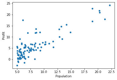
把数据用散点图画出来看一看,kind是scatter就是散点图：

data.plot(kind='scatter', x='Population', y='Profit')
plt.show()

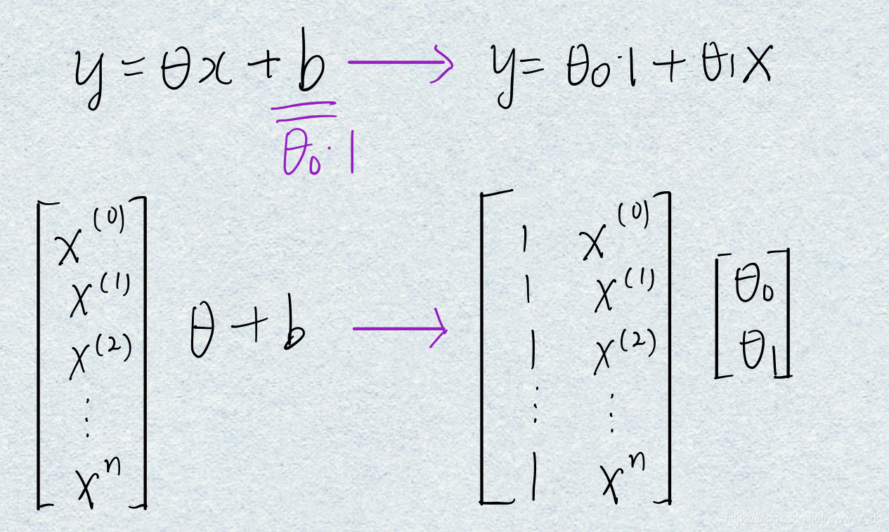
在X第一列插入一列，名字是ones，数据全是1

#如果使用iloc只选择了单独的一行会返回 Series 类型
#如果选择了多行数据则会返回 DataFrame 类型，
data.insert(0, 'Ones', 1)

y = data.iloc[:,2:3]与y = data.iloc[:,2]得到的也是不一样的类型

为什么要在X前面加1:
b是偏置，如果不加偏置b，建立的模型就只是经过原点的直线、平面等。
把截距b和斜率theta统一到一个框架下，就可以通过调整theta0来调整偏置b。

根据代价函数算出当前的参数也就是theta的误差；

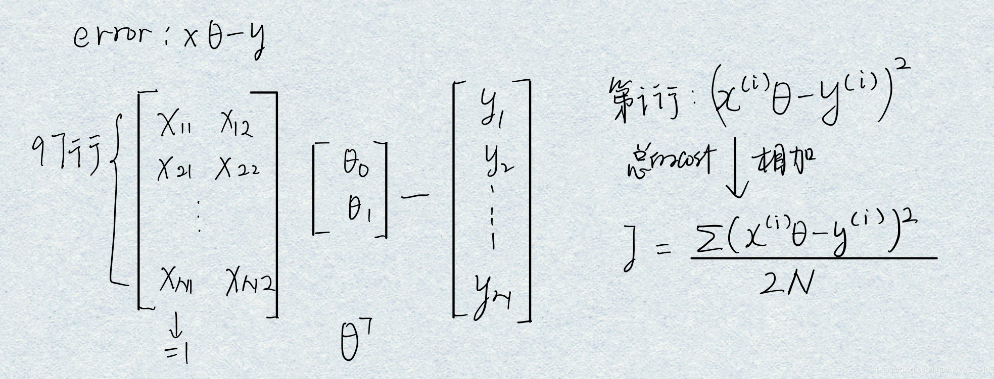
编写代价函数。

def computeCost(X, y, theta):
    inner = np.power(((X * theta.T) - y), 2) #对第一个参数平方
    return np.sum(inner) / (2 * len(X)) #把矩阵的每一个元素加起来

计算一下初始的cost，也就是theta都为0的时候

computeCost(X, y, theta)

32.072733877455676

然后使用梯度下降法优化参数，也就是找到使代价函数最小的theta。
所以现在要求出梯度，对两个参数求导；然后迭代更新theta：

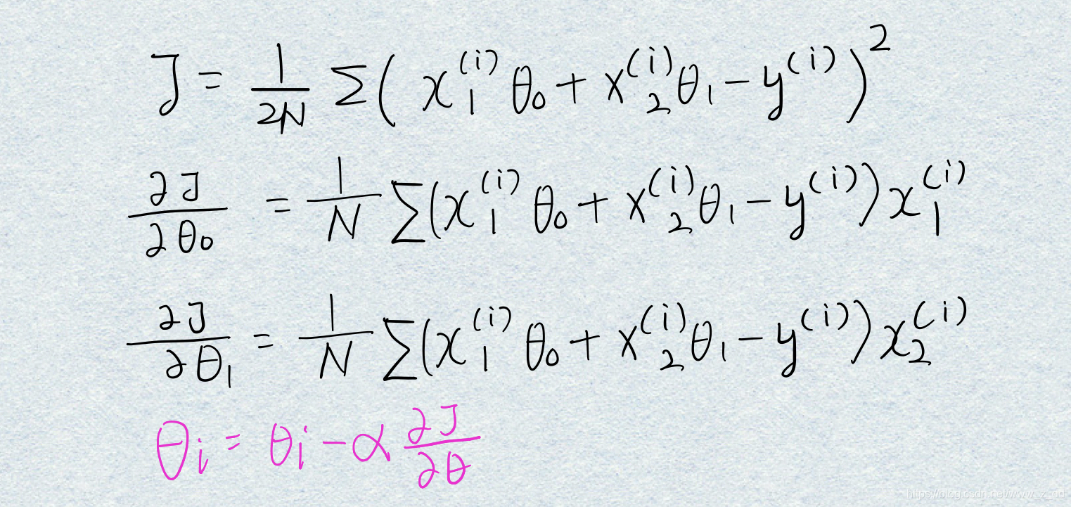
def gradientDescent(X, y, theta, alpha, iters):
    temp = np.matrix(np.zeros(theta.shape))
    parameters = int(theta.ravel().shape[1])
    cost = np.zeros(iters) #保存每一次迭代的cost
    
    for i in range(iters):
        error = (X * theta.T) - y
        for j in range(parameters): #一共有两列，对这两个参数更新
           #  np.multiply(error, X[:,j]) #两个N*1的矩阵对应的点相乘
            temp[0,j] = theta[0,j] - ((alpha / len(X)) * np.sum( np.multiply(error, X[:,j])))
        theta=temp
        cost[i] = computeCost(X, y, theta)
        
    return theta, cost

g, cost = gradientDescent(X, y, theta, 0.01, 1000)

computeCost(X, y, g)

4.515955503078912

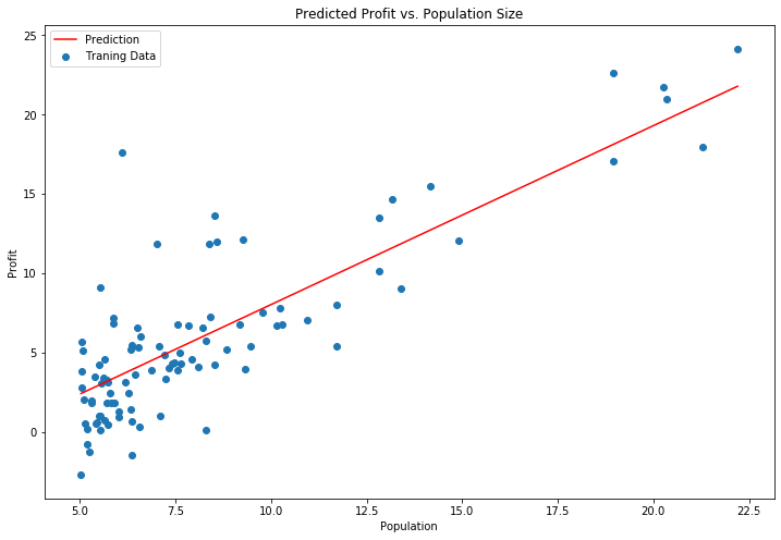
绘制刚刚建立的模型，就是一条直线

x = np.linspace(data.Population.min(), data.Population.max(), 100)
f = g[0, 0] + (g[0, 1] * x)

#把函数F画出来
fig, ax = plt.subplots(figsize=(12,8))
ax.plot(x, f, 'r', label='Prediction')
ax.scatter(data.Population, data.Profit, label='Traning Data')
ax.legend(loc=2)
ax.set_xlabel('Population')
ax.set_ylabel('Profit')
ax.set_title('Predicted Profit vs. Population Size')
plt.show()

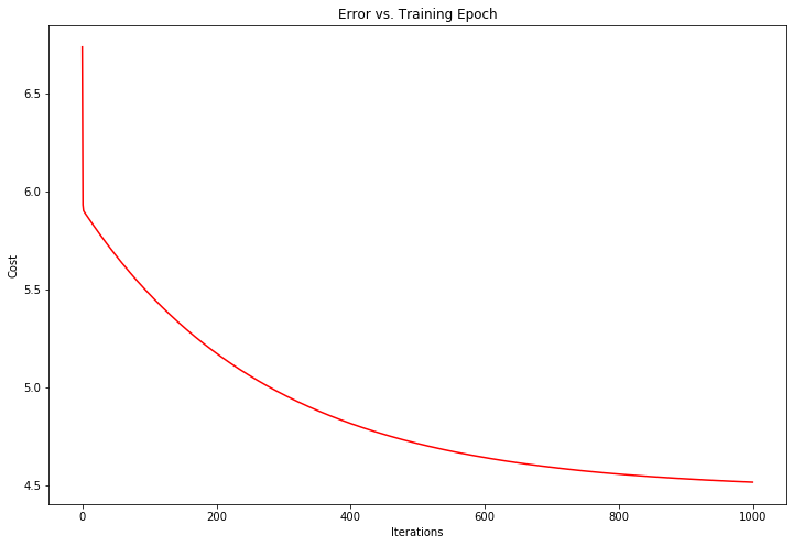
fig, ax = plt.subplots(figsize=(12,8))
ax.plot(np.arange(1000), cost, 'r')
ax.set_xlabel('Iterations')
ax.set_ylabel('Cost')
ax.set_title('Error vs. Training Epoch')
plt.show()

#随着迭代次数的增加，cost越来越小

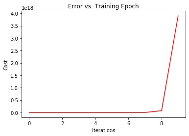
改变learning rate的值看一下

theta = np.matrix(np.array([0,0]))
g, cost = gradientDescent(X, y, theta, 0.1, 10)
fig, ax = plt.subplots(figsize=(6,4))
ax.plot(np.arange(10), cost, 'r')
ax.set_xlabel('Iterations')
ax.set_ylabel('Cost')
ax.set_title('Error vs. Training Epoch')
plt.show()

#随着迭代次数的增加，cost越来越小

二
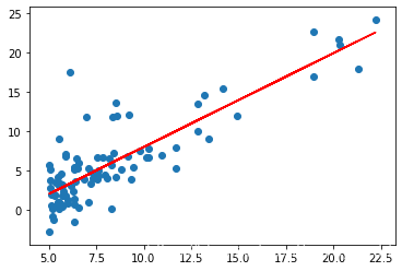
使用scikit-learn的线性回归函数，而不是从头开始实现这些算法。

from sklearn import linear_model
model = linear_model.LinearRegression()
model.fit(X, y)

x = np.array(X[:, 1].A1)
f = model.predict(X).flatten()

fig, ax = plt.subplots(figsize=(6,4))
ax.plot(x, f, 'r', label='Prediction')
#绘制模型
ax.scatter(data.Population, data.Profit, label='Traning Data')
#绘制数据的散点图
plt.show()

三
正规方程求解
只适用于线性模型，如果特征数量n较大则运算代价大，因为矩阵逆的计算时间复杂度为 𝑂(𝑛3) ，通常来说当 𝑛 小于10000 时还是可以接受的。

final_theta2=np.linalg.inv(X.T@X)@X.T@y
final_theta2

matrix([[-3.89578088],
        [ 1.19303364]])

`