


 本文详细介绍使用PyTorch进行深度学习的实践方法,包括线性回归、逻辑回归、卷积神经网络等内容,并通过具体代码示例展示了模型训练流程。
原文链接:PyTorch深度学习实践
刘二大人的课程学习笔记+代码:错错莫
目录
(一)课程概述
本章知识部分涉及到计算图的正向传播(表达式计算)和反向传播(表达式求导),无需赘述。
(二)线性模型
-
机器学习的过程
训练时如果y值已知的学习是监督学习。
数据分为训练集(用于学习)和测试集(用于比对)。
在训练过程中,为了避免过拟合,将训练集中的一部分划分为开发集。
-
样本函数、损失函数(课程笔记已经记录)

-
课程代码:
import numpy as np
import matplotlib.pyplot as plt
from mpl_toolkits.mplot3d import Axes3D

x_data = [1.0, 2.0, 3.0]
y_data = [2.0, 4.0, 6.0]

'''
# y = x*w
def forward(x):
    return x * w

def loss(x,y):
    y_pred = forward(x)
    return (y_pred -y) * (y_pred - y)

w_list = []
mse_list = []
for w in np.arange(0.0,4.1,0.1):
    print('w = ',w)
    l_sum = 0
    for x_val,y_val in zip(x_data,y_data):
        y_pred_val = forward(x_val)
        loss_val = loss(x_val,y_val)
        l_sum += loss_val
        print('\t',x_val,y_val,y_pred_val,loss_val)

    print('MSE = ',l_sum / 3)
    w_list.append(w)
    mse_list.append(l_sum / 3)

#draw the garph
plt.plot(w_list,mse_list)
plt.ylabel('Loss')
plt.xlabel('w')
plt.show()
'''


# y = x*w + b

def forward(x, w, b):
    return x * w + b


def loss(x, y, w, b):
    y_pred = forward(x, w, b)
    return (y_pred - y) * (y_pred - y)


def mse(w, b):
    l_sum = 0
    for x_val, y_val in zip(x_data, y_data):
        y_pred_val = forward(x_val, w, b)
        loss_val = loss(x_val, y_val, w, b)
        l_sum += loss_val
        print('\t', x_val, y_val, y_pred_val, loss_val)
    print('MSE=', l_sum / 3)
    return l_sum / 3


mse_list = []
w = np.arange(0.0, 4.1, 0.1)
b = np.arange(0.0, 4.1, 0.1)
# 生成网格数据
W, B = np.meshgrid(w, b)

Z = mse(W, B)
# draw the garph
figure = plt.figure()
ax = Axes3D(figure)

ax.plot_surface(W,B,Z,rstride=1,cstride=1,cmap='rainbow')
plt.show()
(三)梯度下降算法
-
核心公式
梯度下降法的本质是贪心法。由于函数是凸函数,可以保证贪心法求解得到的是最优解,此时局部最优解即是全局最优解。
此外,学习率α不能过大,否则可能造成不收敛。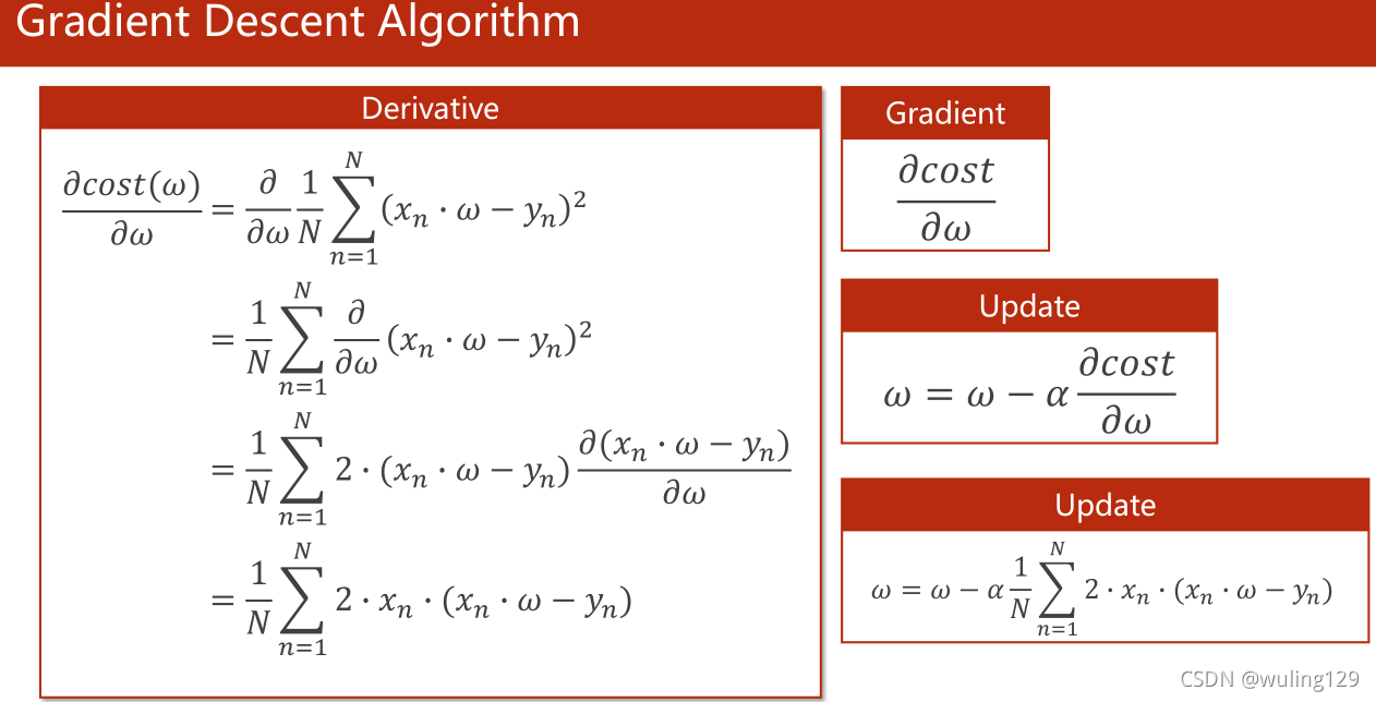
-
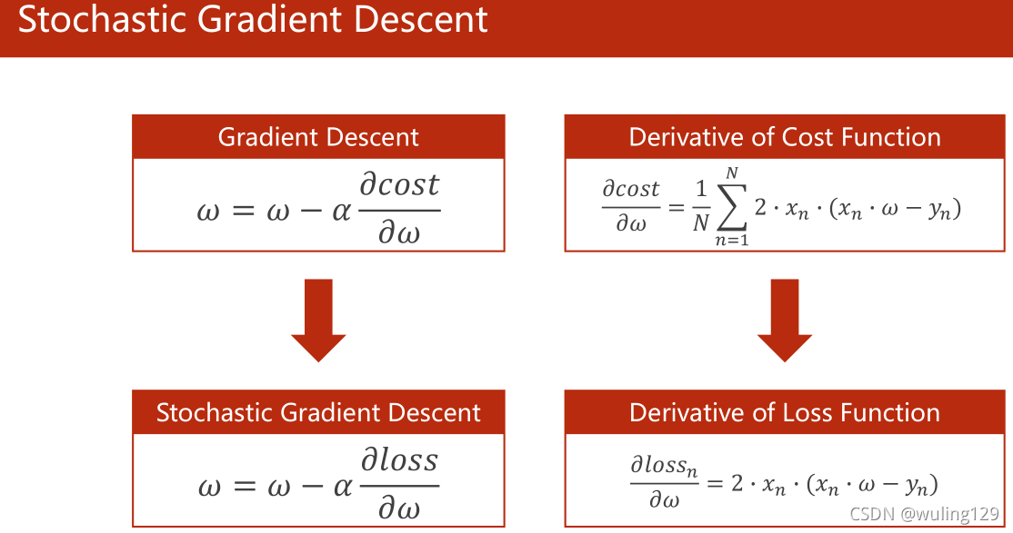
随机梯度下降: 采用单个输入而不是所有输入的均值。梯度下降法计算x(i),x(i+1)的梯度时可以并行计算(因为采用均值),而随机梯度下降法计算x(i),x(i+1)的梯度时w存在前后依赖关系,不能并行。和梯度下降法相比,性能更好但时间复杂度也更高。因此通常采用折中的方案(Batch:批量随机梯度下降)。
-
课程代码
import numpy as np
import matplotlib.pyplot as plt

x_data = [1.0, 2.0, 3.0]
y_data = [2.0, 4.0, 6.0]
w = 1.0


# y = x*w 使用梯度下降计算
def forward(x):
    return x * w


def cost(xs, ys):
    cost = 0
    for x, y in zip(xs, ys):
        y_pred = forward(x)
        cost += (y_pred - y) ** 2
    return cost / len(xs)


def gradient(xs, ys):
    grad = 0
    for x, y in zip(xs, ys):
        grad += 2 * x * (x * w - y)
    return grad / len(xs)


cost_list = []
print("Predict (before trainning)", 4, forward(4))
for epoch in range(100):
    const_val = cost(x_data, y_data)
    cost_list.append(const_val)
    grad_val = gradient(x_data, y_data)
    w -= 0.01 * grad_val
    print("Epoch:", epoch, 'w=', w, 'loss=', const_val)

print("Predict (after trainning)", 4, forward(4))

# draw the garph
x = np.arange(0, 100)
plt.plot(x, cost_list)
plt.ylabel('cost')
plt.xlabel('Epoch')
plt.show()


# SGD stochastic gradient descent
def loss(x, y):
    y_pred = forward(x)
    return (y_pred - y) ** 2


def gradient_sample(x, y):
    return 2 * x * (x * w - y)


w = 1.0
loss_list = []
print("Predict (before trainning)", 4, forward(4))
for epoch in range(100):
    for x, y in zip(x_data, y_data):
        grad = gradient_sample(x, y)
        w = w - 0.01 * grad
        print('\tgrad:', x, y, grad)
        l = loss(x, y)
        loss_list.append(l)

    print("progress: ", epoch, 'w=', w, 'loss=', l)

print("Predict (after trainning)", 4, forward(4))

# draw the garph
x = np.arange(0, 300)
plt.plot(x, loss_list)
plt.ylabel('loss')
plt.xlabel('Epoch')
plt.show()


#mimi-batch(batch)
(四)反向传播
- 直观概念
正向传播是从输入向输出计算,反向传播是从输出向输入逐步求梯度(本质是求导链式法则)。
得到dL/dx后,x作为输出可以继续向前传播。
图中是一个两层的神经网络,在每层的输出中添加一个非线性函数(此处是sigmoid函数,在吴课程中有介绍)。
- 利用PyTorch构建计算图
PyTorch中,Tensor类是最基本的单元,主要存放 权值w(data) 和损失函数对w的导数 dLoss/dw(grad)。
需要注意的是,grad也是Tensor类型。Tensor类型在运算时会建立计算图,并在反向传播完成后释放计算图。如果单纯地使用x的grad的数值进行计算时,要写成x.grad.data的形式。import torch import matplotlib.pyplot as plt x_data = [1.0, 2.0, 3.0] y_data = [2.0, 4.0, 6.0] ''' # if autograd mechanics are required, the element variable requires_grad of Tensor has # to be set to True y^ = w * x loss = (y^ - y) **2 w = torch.Tensor([1.0]) w.requires_grad = True def forward(x): return x * w def loss(x, y): y_pred = forward(x) return (y_pred - y) ** 2 print('predict (befor training)', 4, forward(4).item()) Epoch_list = [] grad_list = [] for epoch in range(50): for x, y in zip(x_data, y_data): l = loss(x, y) l.backward() print('\tgrad:', x, y, w.grad.item()) w.data = w.data - 0.01 * w.grad.data w.grad.data.zero_() print('process:', epoch, l.item()) grad_list.append(l) Epoch_list.append(epoch) print('predict (after training)', 4, forward(4).item()) # draw the garph plt.plot(Epoch_list, grad_list) plt.ylabel('grad') plt.xlabel('Epoch') plt.show() ''' #assignment to be set to True y^ = w1 * x ** 2 + w2 * x +b # loss = (y^ - y) **2 w1 = torch.Tensor([1.0]) w1.requires_grad = True w2 = torch.Tensor([1.0]) w2.requires_grad = True b = torch.Tensor([1.0]) b.requires_grad = True def forward(x): return w1 * x ** 2 + w2 * x + b def loss(x, y): y_pred = forward(x) return (y_pred - y) ** 2 print('predict (befor training)', 4, forward(4).item()) Epoch_list = [] grad_list = [] for epoch in range(50): for x, y in zip(x_data, y_data): l = loss(x, y) l.backward() print('\tgrad:', x, y, w1.grad.item(),w2.grad.item(),b.grad.item()) w1.data = w1.data - 0.01 * w1.grad.data w2.data = w2.data - 0.01 * w2.grad.data b.data = b.data - 0.01 * b.grad.data w1.grad.data.zero_() w2.grad.data.zero_() b.grad.data.zero_() print('process:', epoch, l.item()) grad_list.append(l) Epoch_list.append(epoch) print('predict (after training)', 4, forward(4).item()) # draw the garph plt.plot(Epoch_list, grad_list) plt.ylabel('grad') plt.xlabel('Epoch') plt.show()
(五)用PyTorch实现线性回归
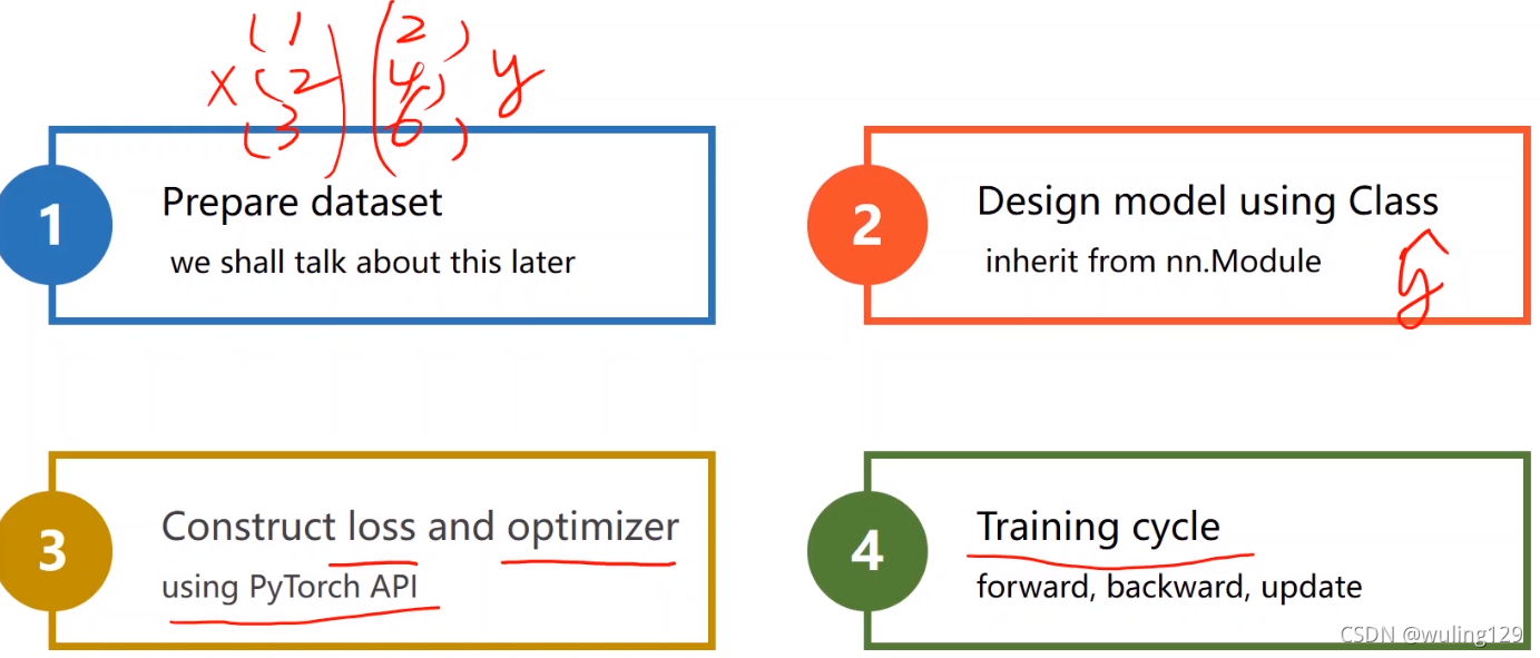
设计步骤:
-准备数据集
-设计模型,计算y的估计值(构造计算图)
-使用PyTorch API构造损失函数、优化器
-训练:前馈算损失、反馈算梯度、更新权值
一个Python传递参数的语法:
实例:
import torch

# Step 1
x_data = torch.Tensor([[1.0], [2.0], [3.0]])
y_data = torch.Tensor([[2.0], [4.0], [6.0]])


# Step 2
class LinearModule(torch.nn.Module):  # 一定要继承自 神经网络模块基类 nn.Module类,并实现__init__()、forward()
    def __init__(self):
        super(LinearModule, self).__init__()
        self.linear = torch.nn.Linear(1, 1)  # 参数分别代表初始的 权值w和偏移b(都是Tensor类)

    def forward(self, x):
        y_pred = self.linear(x)  # linear是Linear类的实例,且该类实现了__call__()方法,在实例化后可以像函数一样调用,通常调用forward()
        return y_pred


model = LinearModule()  # 实例化,model是可调用的
# model(1) 计算x=1时的估计值


# Step 3
#criterion = torch.nn.MSELoss(size_average=False)  # 设置为True也可
criterion = torch.nn.MSELoss(reduction='sum')
optimizer = torch.optim.SGD(model.parameters(), lr=0.01)  # lr即学习率

Epoch_list = []
Cost_list = []

# Step 4
for epoch in range(1000):
    # 前馈
    y_pred = model(x_data)
    loss = criterion(y_pred, y_data)
    print(epoch, loss.data)
    # 反馈
    optimizer.zero_grad()  # 将梯度清零
    loss.backward()
    # 更新
    optimizer.step()

    Cost_list.append(loss)
    Epoch_list.append(epoch)


# 输出结果
print(model.linear.weight.item())  # 输出w
print(model.linear.bias.item())  # 输出b

#draw the garph
plt.plot(Epoch_list,Cost_list)
plt.ylabel('Cost:Adam')
plt.xlabel('Epoch')
plt.show()
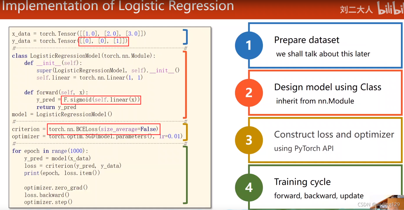
(六)Logistic回归
分类问题
-Logistic回归属于分类问题。分类问题求解是对应情况的概率,并取最大值作为分类结果。
-对于前例,输出由多少分转为能否通过/通过考试的概率。
-使用Logistic函数(标记为σ),将实数空间的输出值映射到 [0,1] 中。此时损失函数也需要改变-(ylog(y’)+(1-y)log(1-y’))。
# 记录LogisticRegressionModel的特点
import torch


class LogisticModel(torch.nn.Module):
    def __init__(self):
        super(LogisticModel, self).__init__()
        self.linear = torch.nn.Linear(1, 1)

    def forward(self, x):
        y_pred = torch.nn.functional.sigmoid(self.linear(x))  # 对原y'进行Sigmoid处理
        return y_pred


criterion = torch.nn.BCELoss(size_average=False)  # 二分类交叉熵,是否取平均值影响学习率大小
(七)多维特征输入的分类问题
-
多维输入的Logistic模型:每个样本对应一个向量,单个样本的输出y’仍然是概率(即y’∈[0,1])。相比一维输入,w*x由实数运算变为向量内积运算。

将N个方程合并成矩阵的运算,利用向量化的特性加速训练过程。
-
Sigmoid函数按向量计算的形式,依次应用到每个元素。

-
分层构造实例

import torch
import numpy as np


xy = np.loadtxt('diabetes.csv.gz', delimiter=',', dtype=np.float32)
x_data = torch.from_numpy(xy[:, :-1])
y_data = torch.from_numpy(xy[:, [-1]])


class MultiDimensionLogisticModel(torch.nn.Module):
    def __init__(self):
        super(MultiDimensionLogisticModel, self).__init__()
        self.linear1 = torch.nn.Linear(8, 6)  # 输入维度为8(每个样本有8个特征),输出维度为6(每个结果有6个特征)
        self.linear2 = torch.nn.Linear(6, 4)
        self.linear3 = torch.nn.Linear(4, 1)  # 经过三层处理最终输出一维
        self.sigmoid = torch.nn.Sigmoid()  # Sigmoid函数为模型添加非线性变换,构建计算图

    def forward(self, x):
        x = self.sigmoid(self.linear1(x))
        x = self.sigmoid(self.linear2(x))
        x = self.sigmoid(self.linear3(x))
        return x


model = MultiDimensionLogisticModel()
criterion = torch.nn.BCELoss(size_average=False)
optimizer = torch.optim.SGD(model.parameters(), lr=0.1)

for epoch in range(1000):
    # 前馈
    y_pred = model(x_data)  # 每次处理所有数据集,而下一章每次处理一个Batch
    loss = criterion(y_pred, y_data)
    print(epoch, loss.data)
    # 反馈
    optimizer.zero_grad()
    loss.backward()
    # 更新
    optimizer.step()
(八)加载数据集
采用DataLoader处理输入时,需要额外定义一个继承自Dataset(该类是抽象类)的类,并实现_init_(), _getitem_(), _len_()方法。
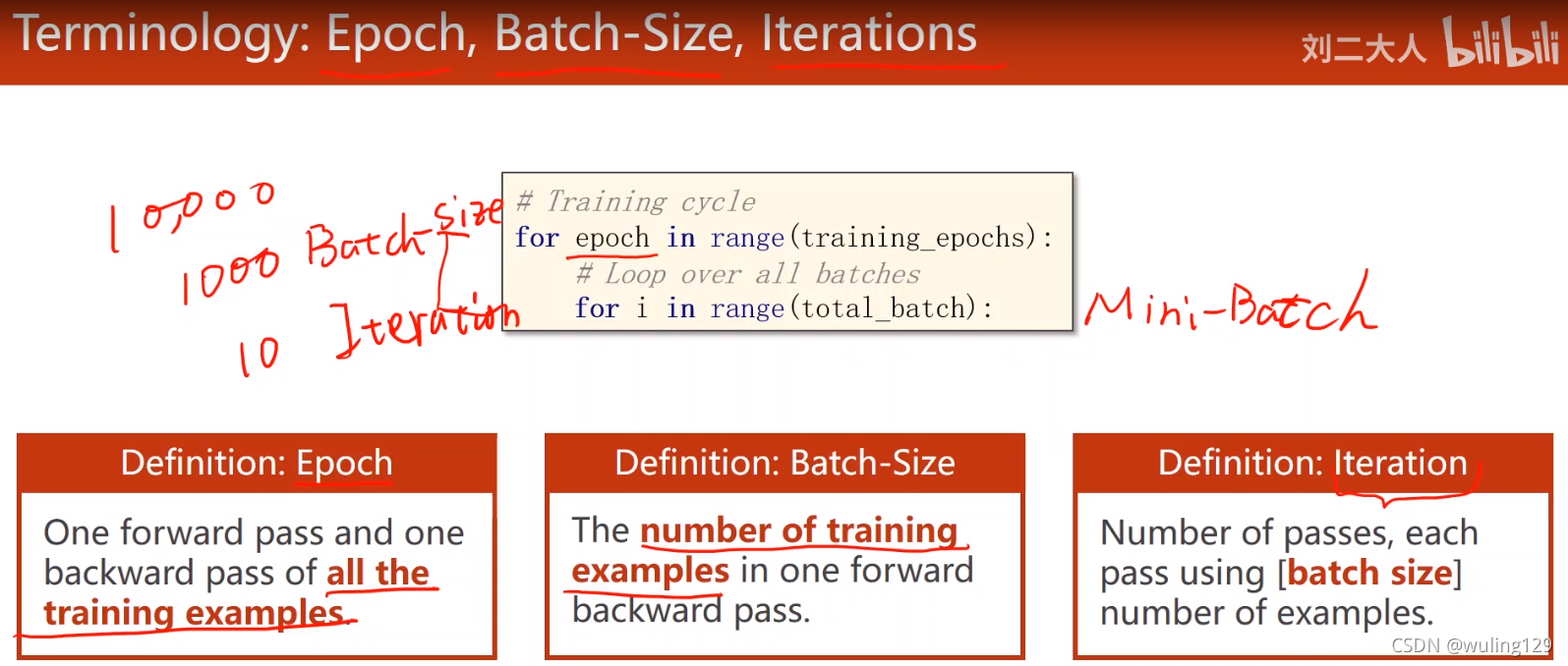
- 概念定义
-Epoch:对所有样本的一次正向传播和反向传播。
-Batch Size:每次正向传播的样本数。
-Iteration:Mini Batch的进行次数。
如:样本数为10000,BatchSize为1000,则Iteration为10
在Mini Batch下的训练步骤:
# Step 4
for epoch in range(training_epochs):  # 对所有数据,共进行training_epochs次的训练
    for i in range(total_batch):  # 对每个Batch进行处理
        #TODO
-
Dataset和DataLoader
DataLoader迭代时以Batch为基本元素,其中Batch的大小在创建Loader时指定。
Dataset每次获取一个样本,DataLoader每次获取Batch个样本。
-
实例
import torch
import numpy as np
from torch.utils.data import Dataset
from torch.utils.data import DataLoader
import matplotlib.pyplot as plt


# Step 1
class DiabetesDataset(Dataset):
    def __init__(self, filepath):
        xy = np.loadtxt(filepath, delimiter=',', dtype=np.float32)
        self.len = xy.shape[0]
        self.x_data = torch.from_numpy(xy[:, :-1])
        self.y_data = torch.from_numpy(xy[:, [-1]])
        self.len = xy.shape[0]  # 和不采用Dataset相比增加的步骤

    def __getitem__(self, index):
        return self.x_data[index], self.y_data[index]

    def __len__(self):
        return self.len


dataset = DiabetesDataset('diabetes.csv.gz')
# dataset是传入数据集,batch_size规定一个batch的样本数,shuffle代表是否打乱样本顺序,num_workers代表并行数目
train_loader = DataLoader(dataset=dataset, batch_size=32, shuffle=True, num_workers=2)


# Step 2(未发生变化)
class MultiDimensionLogisticModel(torch.nn.Module):
    def __init__(self):
        super(MultiDimensionLogisticModel, self).__init__()
        self.linear1 = torch.nn.Linear(8, 6)
        self.linear2 = torch.nn.Linear(6, 4)
        self.linear3 = torch.nn.Linear(4, 1)
        #self.sigmoid = torch.nn.Sigmoid()  # Sigmoid函数为模型添加非线性变换,构建计算图
        self.activate = torch.nn.Sigmoid()

    def forward(self, x):
        x = self.activate(self.linear1(x))
        x = self.activate(self.linear2(x))
        x = self.activate(self.linear3(x))
        return x


model = MultiDimensionLogisticModel()

# Step 3(未发生变化)
#criterion = torch.nn.BCELoss(size_average=False)
criterion = torch.nn.BCELoss(reduction='mean')
#optimizer = torch.optim.SGD(model.parameters(),lr=0.1)
optimizer = torch.optim.Adam(model.parameters(),lr=0.1)

# Step 4

#绘图数据
Epoch_list = []
Cost_list = []

if __name__ == '__main__':
    for epoch in range(100):
        loss_temp = [] #临时记录一次的损失
        for i, data in enumerate(train_loader, 0):  # 每次获取index和一个Batch
            x, y = data  # 其中x和y都是Tensor类型,x代表Batch个输入,y代表Batch个输出
            # 前馈
            y_pred = model(x)
            loss = criterion(y_pred, y)
            print(epoch, i, loss.item())
            # 反馈
            optimizer.zero_grad()
            loss.backward()
            # 更新
            optimizer.step()

            #记录损失
            loss_temp.append(loss.item())

        # save plot graph data
        Cost_list.append(np.sum(loss_temp).item() / len(loss_temp))
        Epoch_list.append(epoch)

    plt.plot(Epoch_list, Cost_list)
    plt.ylabel('loss')
    plt.xlabel('Epoch')
    plt.show()

作业:Build DataLoader for Titanic dataset:
(九)多分类问题
-
Softmax层的引入
相比较二分类问题,多分类需要输出每种情况的对应概率。如果按照二分类的方法,可能造成所有情况概率之和不为1的情况。改进措施是,将输出最终结果前的Sigmoid层转换成Softmax层。

-
引入Softmax层的具体操作
①使用numpy直接计算
import numpy as np

y = np.array([1, 0, 0])  # 标签值
z = np.array([0.2, 0.1, -0.1])  # Softmax输入值
y_pred = np.exp(z)/np.exp(z).sum()
loss = (-y * np.log(y_pred)).sum()
②使用NLLLoss损失函数,输入Softmax和Log处理后的数据,以及标签值,输出Loss。
③使用CrossEntropyLoss(交叉熵损失)函数。
import torch

y = torch.LongTensor([2, 0, 1])  # 注意此处是LongTensor
# z_1和z_2是最后一层输出,进入Softmax之前的值,所以每个分类之和不为1
# 每行元素代表对一个对象的分类情况,共三个对象
z_1 = torch.Tensor([[0.1, 0.2, 0.9],
                    [1.1, 0.1, 0.2],
                    [0.2, 2.1, 0.1]])
z_2 = torch.Tensor([[0.9, 0.2, 0.1],
                    [0.1, 0.1, 0.5],
                    [0.2, 0.1, 0.7]])
criterion = torch.nn.CrossEntropyLoss()
print(criterion(z_1, y), criterion(z_2, y))
- PyTorch图像多分类问题
①数据输入
一般读入形式为whc,在PyTorch中为了便于处理,将其转为cwh。
# 将PIL转为Tensor
transform = transforms.Compose([
    transforms.ToTensor(),
    transforms.Normalize((0.1307, ), (0.3081, ))
])
②设计模型
view将 N个 1维 28*28的输入,转化为 N个 1行 的数据(每行784个)。
注意最后一层不进行激活。
# MNIST

import torch
from torchvision import transforms
from torchvision import datasets
from torch.utils.data import DataLoader
import torch.nn.functional as F
import torch.optim as optim
import matplotlib.pyplot as plt
import numpy as np

#prepare data
batch_size = 64
transform = transforms.Compose([transforms.ToTensor(), transforms.Normalize((0.1307,),(0.3081,)) ]) #conver the PIL image to tesor

train_dataset = datasets.MNIST(root='mnist/', train=True, download=True, transform=transform)
train_loader = DataLoader(train_dataset,shuffle=True,batch_size=batch_size)

test_dataset = datasets.MNIST(root='mnist/', train=False, download=True, transform=transform)
test_loader = DataLoader(test_dataset,shuffle=False,batch_size=batch_size)

# design model
class Net(torch.nn.Module):
    def __init__(self):
        super(Net, self).__init__()
        self.l1 = torch.nn.Linear(784,512)
        self.l2 = torch.nn.Linear(512, 256)
        self.l3 = torch.nn.Linear(256, 128)
        self.l4 = torch.nn.Linear(128, 64)
        self.l5 = torch.nn.Linear(64, 10)

    def forward(self,x):
        x = x.view(-1,784)
        x = F.relu(self.l1(x))
        x = F.relu(self.l2(x))
        x = F.relu(self.l3(x))
        x = F.relu(self.l4(x))
        return  self.l5(x)

model = Net()

#construct loss and optimizer
criterion = torch.nn.CrossEntropyLoss()
optimizer = optim.SGD(model.parameters(),lr=0.01,momentum=0.5)

#training cycle + Test
def train(epoch):
    running_loss = 0.0
    for batch_idx,data in enumerate(train_loader,0):
        inputs, target = data  #对应 x,y
        optimizer.zero_grad()   #优化器清零

        #forward + backward + update
        outputs = model(inputs)
        loss = criterion(outputs,target)
        loss.backward()
        optimizer.step()

        running_loss += loss.item()
        if batch_idx % 300 == 299:
            print('[%d, %5d] loss: %.3f' % (epoch + 1,batch_idx + 1, running_loss / 300))
            running_loss = 0.0


def test():
    correct = 0
    total = 0
    with torch.no_grad():
        for data in test_loader:
            images,labels = data
            outputs = model(images)
            _, predicted = torch.max(outputs.data,dim=1)
            total += labels.size(0)
            correct += (predicted == labels).sum().item()
    print('Accuracy on test set: %d %%' % (100 * correct / total))


if __name__ == '__main__':
    for epoch in range(10):
        train(epoch)
        test()
(十)卷积神经网络
-
图像存储形式
RGB:输入图片是3*w*h的形式,频道对应红/绿/蓝,每个元素取值0~255.
矢量:存储图像的绘制信息。特点是放大不会出现像素块。 -
图像的卷积概述
对图像进行卷积操作,本质上是对图像的某块的所有频道(即一个Batch)进行操作。操作会改变图像的c,w,h值。
-
单通道的卷积操作
用Kernel阵遍历输入阵,对应进行数值乘法再求和,得到输出阵的一个元素。
-
多通道的卷积操作
本质上是将单通道的卷积累加。需要注意的是,输入Kernel的通道数要和输入的通道数相等。
该操作将n通道的输入转化成1通道的输出。
如果需要得到m通道的输出,则要准备m份的卷积阵。此时对应的权值是 m*n*k_width*k_height的四维量。
- 卷积操作实例
import torch

in_channels, out_channels= 5, 10
width, height = 100, 100
kernel_size = 3
batch_size = 1

input = torch.randn(batch_size, in_channels, width, height)
conv_layer = torch.nn.Conv2d(in_channels, out_channels, kernel_size=kernel_size)
output = conv_layer(input)
- 卷积层的Padding操作
在输入阵的周围进行填充(一般是0),以得到目标形状的输出。
import torch

input = [3,4,6,5,7,
         2,4,6,8,2,
         1,6,7,8,4,
         9,7,4,6,2,
         3,7,5,4,1]
input = torch.Tensor(input).view(1, 1, 5, 5)  # 分别对应Batch、Channel、Width、Height
conv_layer = torch.nn.Conv2d(1, 1, kernel_size=3, padding=1, bias=False) # 分别对应输入Channel、输出Channel
kernel = torch.Tensor([1, 2, 3, 4, 5, 6, 7, 8, 9]).view(1, 1, 3, 3)  #输出Channel、输入Channel、Width、Height
conv_layer.weight.data = kernel.data
output = conv_layer(input)
-
步长stride
将上述代码的padding=1改为stride=2,即可得到2*2的结果。 -
Max Pooling层
kernel_size为2的MaxPooling可以将输入的行和列都减少为原来的1/2.
该操作和通道数无关,操作前后不改变通道数。
import torch

input = [3,4,6,5,
         2,4,6,8,
         1,6,7,8,
         9,7,4,6,]
input = torch.Tensor(input).view(1, 1, 4, 4)
maxpooling_layer = torch.nn.MaxPool2d(kernel_size=2)
output = maxpooling_layer(input)
- 卷积神经网络实例
注意:进行最后一次 Conv-Pooling-ReLU后进入线性层。
import torch
import torch.nn.functional as F


class Net(torch.nn.Module):
    def __init__(self):
        super(Net, self).__init__()
        self.conv1 = torch.nn.Conv2d(1, 10, kernel_size=5)  # 卷积层1
        self.conv2 = torch.nn.Conv2d(10, 20, kernel_size=5)  # 卷积层2
        self.pooling = torch.nn.MaxPool2d(2)
        self.linear = torch.nn.Linear(320, 10)  # 输入320个数据,输出10个数据(对应十种分类情况)

    def forward(self, x):
        batch_size = x.size(0)
        x = self.pooling(F.relu(self.conv1(x)))
        x = self.pooling(F.relu(self.conv2(x)))
        x = x.view(batch_size, -1)  # 全连接网络输入
        x = self.linear(x)
        return x


model = Net()
- 使用GPU进行计算
# 在上述代码添加
device = torch.device("cuda:0" if torch.cuda.is_available() else "cpu")
model.to(device)
# 并在训练、测试时,在 input, target = data的基础上增加
input, target = input.to(device), target.to(device)
-
1x1卷积
本质上是将多个通道的对应元素进行信息融合。
目的是,只改变通道数,不改变输入的宽度和高度,以减小运算量。
-
Inception Module
对同一输入进行不同卷积,合并最终结果,取最优解。
不同路径只能改变频道数,不能改变宽度和高度(因为最终需要合并)。
Concatenate操作将不同的卷积结果沿着通道方向合并。
# 上半部分是__init__的操作,下半部分是forward的操作
# 分支1
self.branch_pool = nn.Conv2d(in_channels, 24, kernel_size=1)

branch_pool = F.avg_pool2d(x, kernel_size=3, stride=1, padding=1)
branch_pool = self.branch_pool(branch_pool)

# 分支2
self.branch1x1 = nn.Conv2d(in_channels, 16, kernel_size=1)

branch1x1 = self.branch1x1(x)

# 分支3
self.branch5x5_1 = nn.Conv2d(in_channels,16, kernel_size=1)
self.branch5x5_2 = nn.Conv2d(16, 24, kernel_size=5, padding=2)

branch5x5 = self.branch5x5_1(x)
branch5x5 = self.branch5x5_2(branch5x5)

# 分支4
self.branch3x3_1 = nn.Conv2d(in_channels, 16, kernel_size=1)
self.branch3x3_2 = nn.Conv2d(16, 24, kernel_size=3, padding=1)
self.branch3x3_3 = nn.Conv2d(24, 24, kernel_size=3, padding=1)

branch3x3 = self.branch3x3_1(x)
branch3x3 = self.branch3x3_2(branch3x3)
branch3x3 = self.branch3x3_3(branch3x3)

# Concatenate
outputs = [branch1x1, branch5x5, branch3x3, branch_pool]
return torch.cat(outputs, dim=1)  # (batch, channel, width, height)中channel对应index为1,按照channel对齐
使用实例
import torch
from torch import nn
import torch.nn.functional as F


# 图中的Inception示例
class InceptionA(nn.Module):
    def __init__(self, in_channels):
        super(InceptionA, self).__init__()
        # 定义各分支的卷积部分:
        # 分支2
        self.branch1x1 = nn.Conv2d(in_channels, 16, kernel_size=1)
        # 分支3
        self.branch5x5_1 = nn.Conv2d(in_channels, 16, kernel_size=1)
        self.branch5x5_2 = nn.Conv2d(16, 24, kernel_size=5, padding=2)
        # 分支4
        self.branch3x3_1 = nn.Conv2d(in_channels, 16, kernel_size=1)
        self.branch3x3_2 = nn.Conv2d(16, 24, kernel_size=3, padding=1)
        self.branch3x3_3 = nn.Conv2d(24, 24, kernel_size=3, padding=1)
        # 分支1
        self.branch_pool = nn.Conv2d(in_channels, 24, kernel_size=1)

    def forward(self, x):
        # 分支2
        branch1x1 = self.branch1x1(x)
        # 分支3
        branch5x5 = self.branch5x5_1(x)
        branch5x5 = self.branch5x5_2(branch5x5)
        # 分支4
        branch3x3 = self.branch3x3_1(x)
        branch3x3 = self.branch3x3_2(branch3x3)
        branch3x3 = self.branch3x3_3(branch3x3)
        # 分支1
        branch_pool = F.avg_pool2d(x, kernel_size=3, stride=1, padding=1)
        branch_pool = self.branch_pool(branch_pool)
        # Concatenate
        outputs = [branch1x1, branch5x5, branch3x3, branch_pool]
        return torch.cat(outputs, dim=1)


# 采用Inception的模型
class Net(nn.Module):
    def __init__(self):
        super(Net, self).__init__()
        self.conv1 = nn.Conv2d(1, 10, kernel_size=5)
        self.conv2 = nn.Conv2d(88, 20, kernel_size=5)  # 88是经过Inception1后的通道数
        self.incep1 = InceptionA(in_channels=10)
        self.incep2 = InceptionA(in_channels=20)
        self.mp = nn.MaxPool2d(2)  # pooling操作不改变通道数
        self.linear = nn.Linear(1408, 10)

    def forward(self, x):
        in_size = x.size(0)
        x = F.relu(self.mp(self.conv1(x)))  # 先后进行卷积、池化、激活
        x = self.incep1(x)
        x = F.relu(self.mp(self.conv2(x)))
        x = self.incep2(x)
        x = x.view(in_size, -1)
        x = self.linear(x)
        return x
- Residual Block
不改变输入的c,w,h.
例:进行两次卷积操作的网络
from torch import nn
import torch.nn.functional as F


class ResidualBlock(nn.Module):
    def __init__(self, channel):
        super(ResidualBlock, self).__init__()
        self.conv1 = nn.Conv2d(channel, channel, kernel_size=3, padding=1)
        self.conv2 = nn.Conv2d(channel, channel, kernel_size=3, padding=1)

    def forward(self, x):
        y = F.relu(self.conv1(x))
        y = self.conv2(y)  # 注意此处需要求和后再激活
        y = F.relu(x + y)
        return y


class Net(nn.Module):
    def __init__(self):
        super(Net, self).__init__()
        self.conv1 = nn.Conv2d(1, 16, kernel_size=5)
        self.conv2 = nn.Conv2d(16, 32, kernel_size=5)
        self.mp = nn.MaxPool2d(2)

        self.rblock1 = ResidualBlock(16)
        self.rblock2 = ResidualBlock(32)

        self.linear = nn.Linear(512, 10)

    def forward(self, x):
        in_size = x.size(0)
        x = self.mp(F.relu(self.conv1(x)))
        x = self.rblock1 (x)
        x = self.mp(F.relu(self.conv2(x)))
        x = self.rblock2 (x)
        x = x.view(in_size, -1)
        x = self.linear(x)
        return x
(十一)循环神经网络
-
RNN用于处理输入具有序列关系,且前项对后项有影响的问题。比如根据前几天的温度、气压、天气对未来的天气进行预测。

-
RNNCell
本质是线性层。同一个Cell在RNN中循环使用。
构造RNNCell需要输入inputSize和hiddenSize。
使用时需要明确输入、输出的维度关系。
设 batchSize=1,seqLen=3,inputSize=4,hiddenSize=2
则有 input.shape=(batchSize, inputSize),output.shape=(batchSize, hiddenSize),dataset.shape=(seqLen, batchSize, inputSize)
import torch

batch_size = 1
seq_len = 3
input_size = 4
hidden_size = 2
cell = torch.nn.RNNCell(input_size=input_size, hidden_size=hidden_size)

dataset = torch.randn(seq_len, batch_size, input_size)
hidden = torch.zeros(batch_size, hidden_size)
- RNN

input.shape=(seqLen, batchSize, inputSize)
h0.shape=(numLayers, batchSize, hiddenSize)
output.shape=(seqLen, batchSize, hiddenSize)
hn.shape=(numLayers, batchSize, hiddenSize)
import torch


batch_size = 1
seq_len = 3
input_size = 4
hidden_size = 2
num_layers = 1
cell = torch.nn.RNN(input_size=input_size, hidden_size=hidden_size, num_layers=num_layers)

inputs = torch.randn(seq_len, batch_size, input_size)
hidden = torch.zeros(num_layers, batch_size, hidden_size)
- 实例:使用RNNCell的字符串转化
对于每个输入字符,求解问题的整体结构:
将字符串"hello"转化为"ohlol"
首先将输入字符的每个字符进行向量化,得到RNNCell的输入。
此时inputSize=4,seqLen=5。
# 处理单个字符输入的RNNCell

import torch

# 处理输入
input_size = 4
hidden_size = 4
batch_size = 1
idx2char = ['e', 'h', 'l', 'o']
x_data = [1, 0, 2, 2, 3]  # 'hello'
y_data = [3, 1, 2, 3, 2]  # 'ohlol'
one_hot_lookup = [[1, 0, 0, 0],
                  [0, 1, 0, 0],
                  [0, 0, 1, 0],
                  [0, 0, 0, 1]]
x_one_hot = [one_hot_lookup[x] for x in x_data]  # 得到RNNCell的输入

inputs = torch.Tensor(x_one_hot).view(-1, batch_size, input_size)  # input.shape=(seqLen, batchSize, inputSize)
labels = torch.LongTensor(y_data).view(-1, 1)  # labels.shape=(seqLen, 1)


# 处理单个字符输入的RNNCell
class Model(torch.nn.Module):
    def __init__(self, input_size, hidden_size, batch_size):
        super(Model, self).__init__()
        self.batch_size = batch_size
        self.input_size = input_size
        self.hidden_size = hidden_size
        self.rnncell = torch.nn.RNNCell(input_size=self.input_size, hidden_size=self.hidden_size)

    def forward(self, input, hidden):
        hidden = self.rnncell(input, hidden)  # input.shape=(batchSize, inputSize); hidden.shape=(batch, hiddenSize)
        return hidden

    def init_hidden(self):
        return torch.zeros(self.batch_size, self.hidden_size)  # h0


net = Model(input_size, hidden_size, batch_size)


criterion = torch.nn.CrossEntropyLoss()
optimizer = torch.optim.Adam(net.parameters(), lr=0.1)

for epoch in range(15):
    loss = 0
    optimizer.zero_grad()
    hidden = net.init_hidden()
    print('Predicted string: ',end='')
    # 每轮对所有输入进行训练
    # inputs.shape=(𝒔𝒆𝒒𝑳𝒆𝒏, 𝒃𝒂𝒕𝒄𝒉𝑺𝒊𝒛𝒆,𝒊𝒏𝒑𝒖𝒕𝑺𝒊𝒛𝒆) ; input.shape(𝒃𝒂𝒕𝒄𝒉𝑺𝒊𝒛𝒆, 𝒉𝒊𝒅𝒅𝒆𝒏𝑺𝒊𝒛𝒆)
    for input, label in zip(inputs, labels):
        hidden = net(input, hidden)
        loss += criterion(hidden, label)  # 需要构建计算图,因此需要求和
        _,idx = hidden.max(dim=1)
        print(idx2char[idx.item()],end='')
    loss.backward()
    optimizer.step()
    print(',Epoch [%d/15] loss=%.4f'%(epoch+1,loss.item()))
- 实例:使用RNN的字符串转化
# 处理单个字符输入的RNN
import torch

# 处理输入
num_layers = 1
input_size = 4
hidden_size = 4
batch_size = 1
seq_len = 5
idx2char = ['e', 'h', 'l', 'o']
x_data = [1, 0, 2, 2, 3]  # 'hello'
y_data = [3, 1, 2, 3, 2]  # 'ohlol'
one_hot_lookup = [[1, 0, 0, 0],
                  [0, 1, 0, 0],
                  [0, 0, 1, 0],
                  [0, 0, 0, 1]]
x_one_hot = [one_hot_lookup[x] for x in x_data]  # 得到RNNCell的输入

inputs = torch.Tensor(x_one_hot).view(seq_len, batch_size, input_size)
labels = torch.LongTensor(y_data)  # (seqLen*batchSize, 1)


# 处理单个字符输入的RNNCell
class Model(torch.nn.Module):
    def __init__(self, input_size, hidden_size, batch_size,num_layers=1):
        super(Model, self).__init__()
        self.num_layers = num_layers
        self.batch_size = batch_size
        self.input_size = input_size
        self.hidden_size = hidden_size
        self.rnn = torch.nn.RNN(input_size=self.input_size, hidden_size=self.hidden_size,num_layers=self.num_layers)

    def forward(self, input):
        hidden = torch.zeros(self.num_layers,self.batch_size,self.hidden_size)
        out,_ = self.rnn(input,hidden)
        return out.view(-1,self.hidden_size)


net = Model(input_size, hidden_size, batch_size,num_layers)

criterion = torch.nn.CrossEntropyLoss()
optimizer = torch.optim.Adam(net.parameters(), lr=0.05)

for epoch in range(15):
    optimizer.zero_grad()
    outputs = net(inputs)
    loss = criterion(outputs, labels)
    loss.backward()
    optimizer.step()

    _, idx = outputs.max(dim=1)
    idx = idx.data.numpy()

    print('Predicted: ', ''.join([idx2char[x] for x in idx]),end='')
    print(',Epoch [%d/15] loss=%.3f' % (epoch + 1, loss.item()))
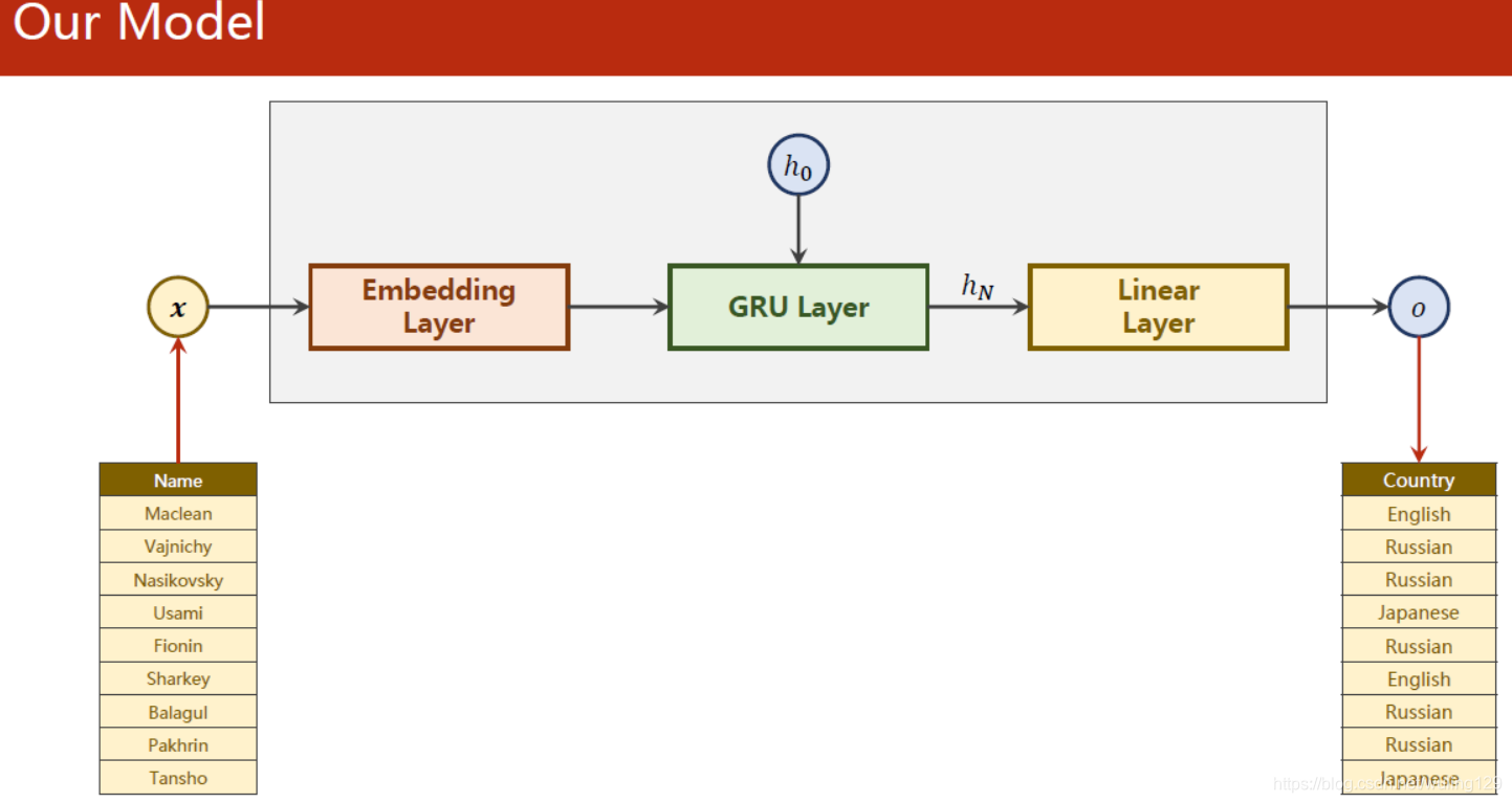
十二、RNN Classifier
代码实现:
# 处理单个字符输入的RNN
import torch
import time
import numpy as np
import math
import matplotlib.pyplot as plt
import gzip
import csv
from torch.utils.data import DataLoader
from torch.nn.utils.rnn import pack_padded_sequence
# 处理输入
HIDDEN_SIZE = 100
BATCH_SIZE = 256
N_LAYER = 2
E_EPOCHS = 100
N_CHARS = 128
USE_GPU = False
#-------------------------------------------------------------------------------------
#prepare data
class NameDataset():
def __init__(self, is_train_set=True):
filename = 'data/names_train.csv.gz' if is_train_set else 'data/names_test.csv.gz'
with gzip.open(filename,'rt') as f:
reader = csv.reader(f)
rows = list(reader)
self.names =[row[0] for row in rows]
self.len = len(self.names)
self.countries = [row[1] for row in rows]
self.country_list = list(sorted(set(self.countries)))
self.country_dict = self.getCountryDict()
self.country_num = len(self.country_list)
def __getitem__(self, index):
return self.names[index], self.country_dict[self.countries[index]]
def __len__(self):
return self.len
def getCountryDict(self):
country_dict = dict()
for idx,country_name in enumerate(self.country_list,0):
country_dict[country_name] = idx
return country_dict
def idx2country(self,index):
return self.country_list[index]
def getCountriesNum(self):
return self.country_num
trainset = NameDataset(is_train_set = True)
trainloader = DataLoader(trainset,batch_size= BATCH_SIZE, shuffle = True)
testset = NameDataset(is_train_set = False)
testloader = DataLoader(testset,batch_size= BATCH_SIZE, shuffle = True)
N_COUNTRY = trainset.getCountriesNum()
#-------------------------------------------------------------------------------------
# 采用 循环卷积神经网络
class RNNClassifier(torch.nn.Module):
def __init__(self, input_size, hidden_size,output_size,n_layers=1,bidirectional=True):
super(RNNClassifier, self).__init__()
self.hiddzen_size =hidden_size
self.n_layers = n_layers
self.n_directions = 2 if bidirectional else 1
self.embedding = torch.nn.Embedding(input_size,hidden_size)
self.gru = torch.nn.GRU(hidden_size,hidden_size,n_layers,bidirectional=bidirectional)
self.fc = torch.nn.Linear(hidden_size*self.n_directions,output_size)
def __int__hidden(self,batch_size):
hidden = torch.zeros(self.n_layers*self.n_directions,batch_size,self.hiddzen_size)
return create_tensor(hidden)
def forward(self,input,seq_lengths):
#input shap:BXS ->SXB
input = input.t()
batch_size = input.size(1)
hidden = self.__int__hidden(batch_size)
embedding = self.embedding(input)
#pack them up
gru_input = pack_padded_sequence(embedding,seq_lengths)
output,hidden = self.gru(gru_input,hidden)
if self.n_directions ==2:
hidden_cat = torch.cat([hidden[-1],hidden[-2]],dim=1)
else:
hidden_cat = hidden[-1]
fc_output = self.fc(hidden_cat)
return fc_output
#--------------------------------------------------------------------------------------------
def make_tensor(names,countries):
sequences_and_lengths = [name2list(name) for name in names]
name_sequences = [s1[0] for s1 in sequences_and_lengths]
seq_lengths = torch.LongTensor([s1[1] for s1 in sequences_and_lengths])
countries = countries.long()
#make tensor of name,BatchSize x seqlen
seq_tensor = torch.zeros(len(name_sequences),seq_lengths.max()).long()
for idx,(seq,seq_len) in enumerate(zip(name_sequences,seq_lengths),0):
seq_tensor[idx, :seq_len] = torch.LongTensor(seq)
#sort by length to use pack_padded_sequence
seq_lengths, perm_idx = seq_lengths.sort(dim=0,descending = True)
seq_tensor = seq_tensor[perm_idx]
countries = countries[perm_idx]
return create_tensor(seq_tensor), create_tensor(seq_lengths), create_tensor(countries)
#计算当前时间距离 起始时间过去多长时间 分钟:秒
def time_since(since):
s = time.time() - since
m = math.floor(s / 60)
s -= m * 60
return '%dm %ds'%(m,s)
def name2list(name):
arr = [ord(c) for c in name]
return arr,len(arr)
def create_tensor(tensor):
if USE_GPU:
device = torch.device("cuda:0")
tensor = tensor.to(device)
return tensor
def trainModel():
total_loss = 0
for i,(names, countries) in enumerate(trainloader,1):
inputs, seq_lengths, target = make_tensor(names,countries)
output = classifier(inputs,seq_lengths)
loss = criterion(output,target)
optimizer.zero_grad()
loss.backward()
optimizer.step()
total_loss += loss.item()
if i%10 == 0:
print(f'[{time_since(start)}] Epoch {epoch}', end='')
print(f'[{i * len(inputs)}/{len(trainset)}]', end='')
print(f'loss ={total_loss/ (i*len(inputs))}')
return total_loss
def testModel():
correct = 0
total = len(testset)
print("evaluating trained model。。。")
with torch.no_grad():
for i,(names, countries) in enumerate(testloader,1):
inputs, seq_lengths, target = make_tensor(names, countries)
output = classifier(inputs, seq_lengths)
pred = output.max(dim=1,keepdim=True)[1]
correct += pred.eq(target.view_as(pred)).sum().item()
percent = '%.2f' % (100 * correct/total)
print(f'Test set: Accuracy {correct}/{total} {percent}%')
return correct /total
if __name__ == '__main__':
classifier = RNNClassifier(N_CHARS,HIDDEN_SIZE,N_COUNTRY,N_LAYER)
if USE_GPU:
device = torch.device("cuda:0")
classifier.to(device)
# construct loss and optimizer
criterion = torch.nn.CrossEntropyLoss()
optimizer = torch.optim.Adam(classifier.parameters(),lr=0.001)
# training cycle + Test
start = time.time()
print("Training for %d epochs..." % E_EPOCHS)
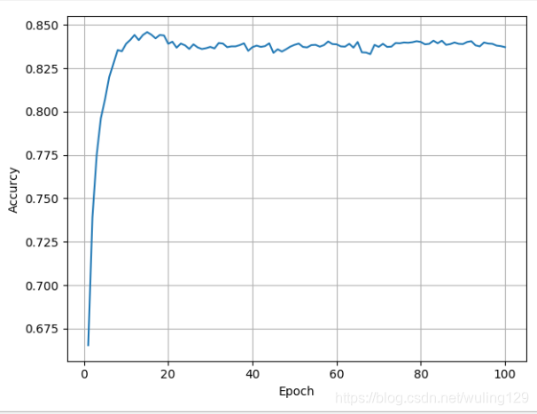
acc_list = []
for epoch in range(1, E_EPOCHS + 1):
#train cycle
trainModel()
acc = testModel()
acc_list.append(acc)
epoch = np.arange(1,len(acc_list)+1,1)
acc_list = np.array(acc_list)
plt.plot(epoch,acc_list)
plt.xlabel('Epoch')
plt.ylabel('Accurcy')
plt.grid()
plt.show()
运行结果:


 1192
1192

 被折叠的 条评论
为什么被折叠?
被折叠的 条评论
为什么被折叠?
 到【灌水乐园】发言


