


二次整合发放(QIF)模型
目录
0. 写在前面
1. QIF 模型的定义
2. QIF 模型的动力学性质
3.
θ
\theta
θ 神经元模型
4. 基于 BrainPy 的 QIF 模型
5. QIF 模型的优点和不足
5.1. QIF 模型的优点
5.2. QIF 模型的不足
6. 思考与总结
0. 写在前面
前面介绍了Hodgkin-Huxley Model和简化神经元模型1 – LIF Model
下面继续介绍简化神经元模型,本篇博客主要是介绍二次整合发放(Quadratic Integrate-and-Fire, QIF)模型,并用BrainPy实现模型的定义、模拟和分析。
前面介绍的LIF Model在动作点位表征上有一定的缺陷,为了弥补这一缺陷,Latham 等人于 2000 年提出了二次整合发放模型(Quadratic Integrate-and-Fire model,QIF model)。
1. QIF 模型的定义
在 QIF 模型中,微分方程右侧的二阶项使得神经元能产生和真实神经元更“像”的动作电位,
具体动力学方程如下:
τ
d
V
d
t
=
a
0
(
V
−
V
rest
)
(
V
−
V
c
)
+
R
I
(
t
)
(1)
\tau \frac{dV}{dt} = a_0 (V - V_{\text{rest}}) (V - V_c) + RI(t) \tag{1}
τdtdV=a0(V−Vrest)(V−Vc)+RI(t)(1)
if
V
>
θ
,
V
←
V
reset
last
t
ref
(2)
\text{if } V > \theta, \quad V \leftarrow V_{\text{reset}} \text{ last } t_{\text{ref}} \tag{2}
if V>θ,V←Vreset last tref(2)
方程 (1)中要求
a
0
>
0
a_0 > 0
a0>0,
V
c
>
V
rest
V_c > V_{\text{rest}}
Vc>Vrest。与LIF模型的动力学方程相比,方程 (1) 右侧是一个关于
V
V
V 的二次方程,这使得膜电位的上升有一个从慢到快的过程,与真实的膜电位变化更加接近。
其中:
- V c V_c Vc 决定了神经元的兴奋阈值。
- a 0 a_0 a0 控制了神经元的发放频率和发放前膜电位的增长速度。
- 当膜电位达到峰值 θ \theta θ 时,神经元发放动作电位,膜电位将被重置为 V reset V_{\text{reset}} Vreset 并进入不应期 t ref t_{\text{ref}} tref。
2. QIF 模型的动力学性质
若不考虑不应期且
θ
→
∞
,
V
reset
→
−
∞
\theta \to \infty, V_{\text{reset}} \to -\infty
θ→∞,Vreset→−∞,且外部电流输入
I
(
t
)
I(t)
I(t) 为常值
I
I
I 的情况下,QIF 微分方程的通解为(笔者没有解出来,借鉴的相关资料):
V
=
V
rest
+
V
c
2
+
R
I
−
a
0
4
(
V
rest
−
V
c
)
2
a
0
tan
(
t
τ
[
R
I
−
a
0
4
(
V
rest
−
V
c
)
2
]
a
0
)
(3)
V = \frac{V_{\text{rest}} + V_c}{2} + \sqrt{\frac{RI - \frac{a_0}{4}(V_{\text{rest}} - V_c)^2}{a_0}} \tan \left( \frac{t}{\tau} \sqrt{\left[ RI - \frac{a_0}{4}(V_{\text{rest}} - V_c)^2 \right] a_0} \right) \tag{3}
V=2Vrest+Vc+a0RI−4a0(Vrest−Vc)2tan(τt[RI−4a0(Vrest−Vc)2]a0)(3)
该方程展示了 V V V 对时间 t t t 的变化为正切函数:
V = m tan k t + n (4) V = m \tan kt + n \tag{4} V=mtankt+n(4)
式中,
m = R I − a 0 4 ( V rest − V c ) 2 a 0 , k = [ R I − a 0 4 ( V rest − V c ) 2 ] a 0 τ , n = V rest + V c 2 (5) m = \sqrt{\frac{RI - \frac{a_0}{4}(V_{\text{rest}} - V_c)^2}{a_0}}, \quad k = \frac{\sqrt{\left[ RI - \frac{a_0}{4}(V_{\text{rest}} - V_c)^2 \right] a_0}}{\tau}, \quad n = \frac{V_{\text{rest}} + V_c}{2} \tag{5} m=a0RI−4a0(Vrest−Vc)2,k=τ[RI−4a0(Vrest−Vc)2]a0,n=2Vrest+Vc(5)
根据正切函数的周期性,QIF 模型的发放周期为
T = π / k (6) T = \pi / k \tag{6} T=π/k(6)
同时,为保证方程 (3) 中的根式有意义且不为 0(否则 V V V 将不产生周期性变化),应要求
R I − a 0 4 ( V rest − V c ) 2 > 0 RI - \frac{a_0}{4}(V_{\text{rest}} - V_c)^2 > 0 RI−4a0(Vrest−Vc)2>0 ⇒ I > a 0 4 R ( V rest − V c ) 2 (7) \Rightarrow I > \frac{a_0}{4R}(V_{\text{rest}} - V_c)^2 \tag{7} ⇒I>4Ra0(Vrest−Vc)2(7)
对于基强度电流 I θ I_\theta Iθ。当 I ≤ I θ I \leq I_{\theta} I≤Iθ时,神经元将不产生动作电位,且膜电位的稳定值随着电流的增加而增加;当电流超过基强度时神经元才能发放动作电位,且发放频率随电流的增加而增加。若 I = I θ I = I_{\theta} I=Iθ,方程 (3) 右侧的第二项为 0,膜电位将稳定在 V = V rest + V c 2 V = \frac{V_{\text{rest}} + V_c}{2} V=2Vrest+Vc。
下面讨论一下 a 0 a_0 a0与模型发放频率的关系。由方程 (6) 和方程 (5) 可知 QIF 模型的发放频率为
f = k π = − ( V rest − V c ) 2 4 a 0 2 + R I a 0 π τ (8) f = \frac{k}{\pi} = \frac{\sqrt{-\frac{(V_{\text{rest}} - V_c)^2}{4a_0^2} + R I a_0}}{\pi \tau} \quad \tag{8} f=πk=πτ−4a02(Vrest−Vc)2+RIa0(8)
由方程 (7) 及 a 0 > 0 a_0 > 0 a0>0 可以求得 a 0 a_0 a0 的取值范围为 a 0 ∈ ( 0 , 4 R I ( V rest − V c ) 2 ) a_0 \in \left(0, \frac{4RI}{(V_{\text{rest}} - V_c)^2}\right) a0∈(0,(Vrest−Vc)24RI)。由于方程 (8) 根式中的式子是关于 a 0 a_0 a0 的二次函数,根据二次函数性质, f f f 在 ( 0 , 2 R I ( V rest − V c ) 2 ) \left(0, \frac{2RI}{(V_{\text{rest}} - V_c)^2}\right) (0,(Vrest−Vc)22RI)内随 a 0 a_0 a0 单调递增,在 ( 2 R I ( V rest − V c ) 2 , 4 R I ( V rest − c ) 2 ) \left(\frac{2RI}{(V_{\text{rest}} - V_c)^2}, \frac{4RI}{(V_{\text{rest}} -_c)^2}\right) ((Vrest−Vc)22RI,(Vrest−c)24RI)内随 a 0 a_0 a0 单调递减。
为什么一个恒定的外部电流输入 𝐼 要达到基强度后,QIF 模型才能产生动作电位呢?这部分可以可以利用 BrainPy里的一维相平面分析工具画出不同的恒定电流输入下膜电位变化率 d𝑉/d𝑡 与膜电位 𝑉 的关系。由于涉及到代码部分,因此相平面分析的部分放在代码的部分进行讨论。
3. θ \theta θ 神经元模型
对于上述分析的式(1),可以通过数学推导转换成更加简洁的形式。具体而言,将式(1)转化为如下的形式:
d
V
d
t
=
a
0
τ
(
V
−
V
rest
+
V
c
2
)
2
+
a
0
τ
[
V
rest
V
c
−
(
V
−
V
rest
+
V
c
2
)
2
]
+
R
I
(
t
)
τ
(9)
\frac{dV}{dt} = \frac{a_0}{\tau} \left( V - \frac{V_{\text{rest}} + V_c}{2} \right)^2 + \frac{a_0}{\tau} \left[ V_{\text{rest}} V_c - \left( V - \frac{V_{\text{rest}} + V_c}{2} \right)^2 \right] + \frac{RI(t)}{\tau}\tag{9}
dtdV=τa0(V−2Vrest+Vc)2+τa0[VrestVc−(V−2Vrest+Vc)2]+τRI(t)(9)令
x
=
a
0
τ
(
V
−
V
rest
+
V
c
2
)
x = \frac{a_0}{\tau} \left( V - \frac{V_{\text{rest}} + V_c}{2} \right)
x=τa0(V−2Vrest+Vc),则有
τ
a
0
d
x
d
t
=
x
2
+
a
0
τ
[
V
rest
V
c
−
(
V
rest
+
V
c
2
)
2
]
+
R
I
(
t
)
τ
\frac{\tau}{a_0} \frac{dx}{dt} = x^2 + \frac{a_0}{\tau} \left[ V_{\text{rest}} V_c - \left( \frac{V_{\text{rest}} + V_c}{2} \right)^2 \right] + \frac{RI(t)}{\tau}
a0τdtdx=x2+τa0[VrestVc−(2Vrest+Vc)2]+τRI(t)
⇒
d
x
d
t
=
x
2
+
a
0
τ
(
a
0
τ
[
V
rest
V
c
−
(
V
rest
+
V
c
2
)
2
]
+
R
I
(
t
)
τ
)
\Rightarrow \frac{dx}{dt} = x^2 + \frac{a_0}{\tau} \left( \frac{a_0}{\tau} \left[ V_{\text{rest}} V_c - \left( \frac{V_{\text{rest}} + V_c}{2} \right)^2 \right] + \frac{RI(t)}{\tau} \right)
⇒dtdx=x2+τa0(τa0[VrestVc−(2Vrest+Vc)2]+τRI(t))
⇒
d
x
d
t
=
x
2
+
b
I
(
t
)
+
c
(10)
\Rightarrow \frac{dx}{dt} = x^2 + bI(t) + c \quad \tag{10}
⇒dtdx=x2+bI(t)+c(10)其中
b
=
a
0
R
τ
2
b = \frac{a_0 R}{\tau^2}
b=τ2a0R,
c
=
a
0
2
τ
2
(
V
rest
V
c
)
−
(
V
rest
+
V
c
2
)
2
c = \frac{a_0^2}{\tau^2} \left( V_{\text{rest}} V_c \right) - \left( \frac{V_{\text{rest}} + V_c}{2} \right)^2
c=τ2a02(VrestVc)−(2Vrest+Vc)2。令
x
=
1
2
tan
θ
x = \frac{1}{2} \tan \theta
x=21tanθ,代入上式,得到
1
2
cos
2
θ
2
d
θ
d
t
=
tan
2
θ
2
+
b
I
(
t
)
+
c
\frac{1}{2 \cos^2 \frac{\theta}{2}} \frac{d\theta}{dt} = \tan^2 \frac{\theta}{2} + bI(t) + c
2cos22θ1dtdθ=tan22θ+bI(t)+c
⇒
d
θ
d
t
=
2
sin
2
θ
2
+
2
cos
2
θ
2
(
b
I
(
t
)
+
c
)
\Rightarrow \frac{d\theta}{dt} = 2 \sin^2 \frac{\theta}{2} + 2 \cos^2 \frac{\theta}{2} (bI(t) + c)
⇒dtdθ=2sin22θ+2cos22θ(bI(t)+c)
⇒
d
θ
d
t
=
−
cos
θ
+
(
1
+
cos
θ
)
(
2
c
+
1
2
+
2
b
I
(
t
)
)
(11)
\Rightarrow \frac{d\theta}{dt} = -\cos \theta + (1 + \cos \theta) \left( 2c + \frac{1}{2} + 2bI(t) \right) \quad \tag{11}
⇒dtdθ=−cosθ+(1+cosθ)(2c+21+2bI(t))(11)
这便是
θ
\theta
θ 神经元模型(
θ
\theta
θ-Neuron model)的一种数学表示,它和
t
ref
=
0
t_{\text{ref}} = 0
tref=0,
θ
→
∞
\theta \to \infty
θ→∞,
V
reset
→
−
∞
V_{\text{reset}} \to -\infty
Vreset→−∞ 的 QIF 模型等价。
另一种经典表示与方程 (11) 大同小异:
d
θ
d
t
=
1
−
cos
θ
+
(
1
+
cos
θ
)
(
β
+
I
(
t
)
)
(12)
\frac{d\theta}{dt} = 1 - \cos \theta + (1 + \cos \theta) (\beta + I(t)) \quad \tag{12}
dtdθ=1−cosθ+(1+cosθ)(β+I(t))(12)
理论分析可知:
和 QIF 模型相比,经过推导和简化后的 𝜃 神经元模型不再需要显式地重置发放脉冲的神经元,而是通过将 𝜃 限制在 (0, 2π) 的区间上隐式地完成这一操作。后面代码部分会进行详细的分析与说明。
4. 基于BrainPy 的 QIF 模型
下面利用 BrainPy 实现QIF模型,QIF 模型的定义与 LIF 模型相似,只需在初始化函数__init__()中初始化相应的参数,并修改微分方程的表达即可。代码如下:
import brainpy as bp
import brainpy.math as bm
import matplotlib.pyplot as plt

plt.rcParams.update({"font.size": 15})
plt.rcParams['font.sans-serif'] = ['Times New Roman']


class QIF(bp.dyn.NeuDyn):
    def __init__(self, size, V_rest=-65., V_reset=-68., V_th=-0., V_c=-50.0, a_0=.07, R=1., tau=10., t_ref=5.,
                 **kwargs):
        # 初始化父类
        super(QIF, self).__init__(size=size, **kwargs)

        # 初始化参数
        self.V_rest = V_rest
        self.V_reset = V_reset
        self.V_th = V_th
        self.V_c = V_c
        self.a_0 = a_0
        self.R = R
        self.tau = tau
        self.t_ref = t_ref  # 不应期时长

        # 初始化变量
        self.V = bm.Variable(bm.random.randn(self.num) + V_reset)
        self.input = bm.Variable(bm.zeros(self.num))
        self.t_last_spike = bm.Variable(bm.ones(self.num) * -1e7)  # 上一次脉冲发放时间
        self.refractory = bm.Variable(
            bm.zeros(self.num, dtype=bool))  # 是否处于不应期
        self.spike = bm.Variable(bm.zeros(self.num, dtype=bool))  # 脉冲发放状态

        # 使用指数欧拉方法进行积分
        self.integral = bp.odeint(f=self.derivative, method='exp_auto')

    # 定义膜电位关于时间变化的微分方程
    def derivative(self, V, t, Iext):
        dvdt = (self.a_0 * (V - self.V_rest) *
                (V - self.V_c) + self.R * Iext) / self.tau
        return dvdt

    def update(self):
        _t, _dt = bp.share['t'], bp.share['dt']
        # 以数组的方式对神经元进行更新
        refractory = (_t - self.t_last_spike) <= self.t_ref  # 判断神经元是否处于不应期
        V = self.integral(self.V, _t, self.input, dt=_dt)  # 根据时间步长更新膜电位
        # 若处于不应期,则返回原始膜电位self.V,否则返回更新后的膜电位V
        V = bm.where(refractory, self.V, V)
        spike = V > self.V_th  # 将大于阈值的神经元标记为发放了脉冲
        self.spike.value = spike  # 更新神经元脉冲发放状态
        self.t_last_spike.value = bm.where(
            spike, _t, self.t_last_spike)  # 更新最后一次脉冲发放时间
        # 将发放了脉冲的神经元膜电位置为V_reset,其余不变
        self.V.value = bm.where(spike, self.V_reset, V)
        self.refractory.value = bm.logical_or(
            refractory, spike)  # 更新神经元是否处于不应期
        self.input[:] = 0.  # 重置外界输入
在定义好 QIF 模型后,简单地初始化一个 QIF 模型并进行模拟:
def run_QIF():
    # 运行QIF模型
    group = QIF(1)
    runner = bp.DSRunner(
        group, monitors=['V'], inputs=('input', 6.))  # 输入电流的变量和数值
    runner(500)  # 运行时长为500ms
    # 结果可视化
    fig, gs = bp.visualize.get_figure(1, 1, 4.5, 6)
    ax = fig.add_subplot(gs[0, 0])
    plt.plot(runner.mon.ts, runner.mon.V)
    plt.xlabel(r'$t$ (ms)')
    plt.ylabel(r'$V$ (mV)')
    ax.spines['top'].set_visible(False)
    ax.spines['right'].set_visible(False)
    # plt.savefig('QIF_output2.pdf', transparent=True, dpi=500)
    plt.show()
得到的图像如下:

由上图可见,相比 LIF 模型,QIF 模型膜电位随时间变化的曲线和真实情况更加符合。尽管都是对
V
V
V 重置的判断,式 (2) 中的
θ
\theta
θ 和 LIF 模型中
V
th
V_{\text{th}}
Vth 的含义不完全相同:在 LIF 模型中,
V
V
V 达到
V
th
V_{\text{th}}
Vth 后开始发放脉冲(只不过整个动作电位的过程被简化为了重置),而在 QIF 模型中,
θ
\theta
θ 刻画的是脉冲发放过程中膜电位的尖峰值,动作电位在更早的时候就已经开始产生了。
对于上方代码中设定的各个参数,可以求得基强度电流为 I θ = 3.94 I_{\theta} = 3.94 Iθ=3.94。当 I < = 3.94 I <= 3.94 I<=3.94 时,模型将不产生动作电位。
下图给出了不同的恒定电流输入下膜电位随时间的变化。与 LIF 模型相似,当电流小于基强度时,神经元将不产生动作电位,且膜电位的稳定值随着电流的增加而增加;当电流超过基强度时神经元才能发放动作电位,且发放频率随电流的增加而增加。若
I
=
I
θ
I = I_{\theta}
I=Iθ,方程 (3) 右侧的第二项为 0,膜电位将稳定在
V
=
V
rest
+
V
c
2
V = \frac{V_{\text{rest}} + V_c}{2}
V=2Vrest+Vc。

上述图片由下面的代码进行生成:
def QIF_input_threshold():
    def QIF_plot(input, duration, color):
        neu = QIF(1)
        neu.V[:] = bm.array([-68.])
        runner = bp.DSRunner(neu, monitors=['V'], inputs=('input', input))
        runner(duration)
        plt.plot(runner.mon.ts, runner.mon.V, color=color,
                 label='input={}'.format(input))

    inputs = [0., 3., 4., 5.]
    colors = [u'#2ca02c', u'#d62728', u'#1f77b4', u'#ff7f0e']
    dur = 500

    fig, gs = bp.visualize.get_figure(1, 1, 4.5, 6)
    ax = fig.add_subplot(gs[0, 0])
    for i in range(len(inputs)):
        QIF_plot(inputs[i], dur, colors[i])

    plt.text(104, -25, 'input=5.')
    plt.text(462, -25, 'input=4.')
    plt.annotate('input=3.', xy=(144, -61.5), xytext=(110, -45),
                 arrowprops=dict(arrowstyle="->"))
    plt.annotate('input=0.', xy=(237.5, -65.15), xytext=(215, -50),
                 arrowprops=dict(arrowstyle="->"))
    plt.xlabel(r'$t$ (ms)')
    plt.ylabel(r'$V$ (mV)')
    ax.spines['top'].set_visible(False)
    ax.spines['right'].set_visible(False)
    plt.xlim(-1, 541)
    # 设置X轴的最小值为 -1,最大值为 541
    # plt.savefig('QIF_input_threshold.pdf', transparent=True, dpi=500)
    plt.show()
下面使用代码探讨 a 0 a_0 a0与模型发放频率的关系
def a0_effect():
    duration = 500

    fig, gs = bp.visualize.get_figure(3, 1, 1.5, 6)

    neu1 = QIF(1, a_0=0.005)
    neu1.V[:] = bm.array([-68.])
    runner = bp.DSRunner(neu1, monitors=['V'], inputs=('input', 5.))
    runner(duration)
    ax1 = fig.add_subplot(gs[0, 0])
    ax1.plot(runner.mon.ts, runner.mon.V,
             color=u'#d62728', label=r'$a_0$=0.005')
    ax1.set_ylabel(r'$V$ (mV)')
    ax1.legend(loc='upper right')
    ax1.spines['top'].set_visible(False)
    ax1.spines['right'].set_visible(False)

    neu1 = QIF(1, a_0=0.045)
    neu1.V[:] = bm.array([-68.])
    runner = bp.DSRunner(neu1, monitors=['V'], inputs=('input', 5.))
    runner(duration)
    ax2 = fig.add_subplot(gs[1, 0])
    ax2.plot(runner.mon.ts, runner.mon.V,
             color=u'#1f77b4', label=r'$a_0$=0.045')
    ax2.set_ylabel(r'$V$ (mV)')
    ax2.legend(loc='upper right')  # 指定添加的图例的位置在右上角
    ax2.spines['top'].set_visible(False)
    ax2.spines['right'].set_visible(False)

    neu1 = QIF(1, a_0=0.08)
    neu1.V[:] = bm.array([-68.])
    runner = bp.DSRunner(neu1, monitors=['V'], inputs=('input', 5.))
    runner(duration)
    ax3 = fig.add_subplot(gs[2, 0])
    ax3.plot(runner.mon.ts, runner.mon.V,
             color=u'#ff7f0e', label=r'$a_0$=0.08')
    ax3.set_ylabel(r'$V$ (mV)')
    ax3.set_xlabel(r'$t$ (ms)')
    ax3.legend(loc='upper right')
    ax3.spines['top'].set_visible(False)
    ax3.spines['right'].set_visible(False)

    # plt.savefig('QIF_a0.png', transparent=True, dpi=500)
    plt.show()
在之前定义的 QIF 模型中,固定
I
=
5
I = 5
I=5,则
a
0
∈
(
0
,
0.089
)
a_0 \in (0, 0.089)
a0∈(0,0.089)。图3.7展示了
a
0
a_0
a0 的取值对 QIF 神经元发放频率及发放曲线的影响。随着
a
0
a_0
a0 的增长,神经元发放频率先增加后降低。此外,随着
a
0
a_0
a0 的增长,阈下膜电位变化曲线从平滑上升变为先缓慢上升,后急速上升。因此,
a
0
a_0
a0 不仅影响了 QIF 模型的发放频率,还刻画了膜电位的上升曲线。

实际上,在理论分析中,
a
0
=
0.045
a_0 = 0.045
a0=0.045 时发放频率最大,但由于阈值电位和重置电位的存在,上图膜电位变化并没有经历一个完整的正切周期,因此发放频率达到最大值时
a
0
a_0
a0 并不严格等于
2
R
I
(
V
rest
−
V
c
)
2
\frac{2RI (V_{\text{rest}} - V_c)}{2}
22RI(Vrest−Vc),而是低于此值。
前面提到的一维相平面分析,在此使用BrainPy的相关工具进行可视化:
def phase_plane():
    bp.math.enable_x64()  # 启用64位浮点数计算模式

    def phase_plane_analysis(model, I_ext, res=0.005, extra_fun=None):
        fig, gs = bp.visualize.get_figure(1, 1, 3.5, 4.5)
        ax = fig.add_subplot(gs[0, 0])
        pp = bp.analysis.PhasePlane1D(
            model=model,
            target_vars={'V': [-80, -30]},
            pars_update={'Iext': I_ext},
            resolutions=res
        )
        pp.plot_vector_field()
        pp.plot_fixed_point()
        ax.set_xlabel(r'$V$')
        ax.spines['top'].set_visible(False)
        ax.spines['right'].set_visible(False)
        if extra_fun is not None:
            extra_fun()
        ax.get_legend().remove()
        # plt.savefig(f'QIF_I={I_ext}.pdf', dpi=500, transparent=True)

    qif = QIF(1)

    def f():
        plt.annotate('stable point', xy=(-65.0, 0),
                     xytext=(-73, 1.6), arrowprops=dict(arrowstyle="->"))
        plt.annotate('unstable point', xy=(-50.0, 0),
                     xytext=(-53, 1.6), arrowprops=dict(arrowstyle="->"))
        plt.scatter([-70, -45], [0., 0.], marker='4', s=100, color='k')
        plt.scatter([-58, ], [0., ], marker='3', s=100, color='k')
        plt.text(-30, 5, 'I=0.0', fontsize=25,
                 ha='right', va='top', color='purple')

    phase_plane_analysis(qif, 0., extra_fun=f)

    def f():
        plt.annotate('stable point', xy=(-63.977984, 0),
                     xytext=(-73, 1.6), arrowprops=dict(arrowstyle="->"))
        plt.annotate('unstable point', xy=(-51.022015, 0),
                     xytext=(-53, 1.6), arrowprops=dict(arrowstyle="->"))
        plt.scatter([-70, -45], [0., 0.], marker='4', s=100, color='k')
        plt.scatter([-58, ], [0., ], marker='3', s=100, color='k')
        # 右上角加上注释
        plt.text(-30, 5, 'I=1.0', fontsize=25,
                 ha='right', va='top', color='purple')

    phase_plane_analysis(qif, 1., extra_fun=f)

    def f():
        plt.annotate('stable point', xy=(-61.159625, 0),
                     xytext=(-70, 1.6), arrowprops=dict(arrowstyle="->"))
        plt.annotate('unstable point', xy=(-53.84037, 0),
                     xytext=(-55, 1.6), arrowprops=dict(arrowstyle="->"))
        plt.scatter([-70, -45], [0., 0.], marker='4', s=100, color='k')
        plt.scatter([-58, ], [0., ], marker='3', s=100, color='k')
        plt.text(-30, 5, 'I=3.0', fontsize=25,
                 ha='right', va='top', color='purple')

    phase_plane_analysis(qif, 3., extra_fun=f)

    def f():
        plt.scatter([-55], [0.], marker='4', s=100, color='k')
        plt.text(-30, 5, 'I=10.0', fontsize=25,
                 ha='right', va='top', color='purple')

    phase_plane_analysis(qif, 10., extra_fun=f)

    plt.show()
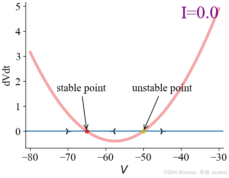
相平面分析结果下图所示。当 I = 0.0 I =0.0 I=0.0 时, d V d t \frac{dV}{dt} dtdV 有两个零点,即 V stable = V rest V_{\text{stable}} = V_{\text{rest}} Vstable=Vrest 和 V unstable = V c V_{\text{unstable}} = V_c Vunstable=Vc,其中 V stable V_{\text{stable}} Vstable 为稳定点(图中“stable point”), V unstable V_{\text{unstable}} Vunstable 为不稳定点(图中“unstable point”)。此时,该模型表现出初始点依赖特性。
- 当初始膜电位 V ( 0 ) < V c V(0) < V_c V(0)<Vc 时,膜电位会逐渐被稳定点所吸引(如图 I = 0.0 I =0.0 I=0.0中箭头所示),直至稳定到 V rest V_{\text{rest}} Vrest;
- 当初始膜电位 V ( 0 ) > V c V(0) > V_c V(0)>Vc 时, V V V 受到不稳定的排斥会不断升高(如图 I = 0.0 I =0.0 I=0.0中箭头所示),直至产生动作电位发放。
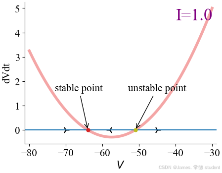
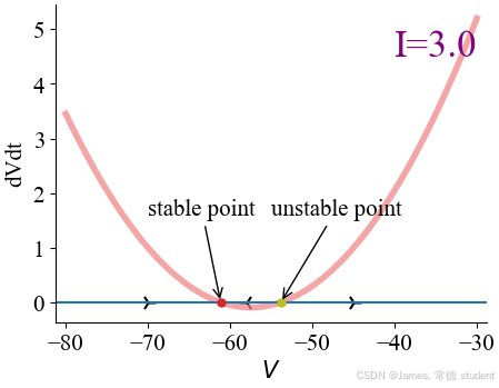
当给予神经元一定电流时,此时模型的相图将发生变化。如图
I
=
1.0
I =1.0
I=1.0、图
I
=
3.0
I =3.0
I=3.0和图
I
=
10.0
I = 10.0
I=10.0所示,
d
V
/
d
t
dV/dt
dV/dt 随着
I
I
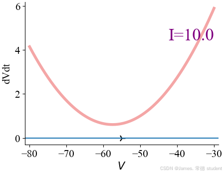
I 的增大而上移。上移过程中,两个不动点逐渐靠近(图
I
=
3.0
I = 3.0
I=3.0),并合并为一个鞍点(saddle point),直至最终消失(图
I
=
10.0
I =10.0
I=10.0)。在动力学系统理论中,我们一般将此过程称为鞍结分岔(saddle-node bifurcation)。
若神经元接受到一个
I
<
I
θ
I < I_\theta
I<Iθ 的恒定电流输入时(图3.8(b)),模型有两个不动点。我们令方程 (3.11) 左侧等于 0,可以求得膜电位的这两个不动点为
V
s
t
a
b
l
e
=
V
r
e
s
t
+
V
c
2
−
1
2
(
V
r
e
s
t
+
V
c
)
2
−
4
R
I
a
0
(13)
V_{stable} = \frac{V_{rest} + V_c}{2} - \frac{1}{2}\sqrt{(V_{rest} + V_c)^2 - \frac{4RI}{a_0}}\tag{13}
Vstable=2Vrest+Vc−21(Vrest+Vc)2−a04RI(13)
V
u
n
s
t
a
b
l
e
=
V
r
e
s
t
+
V
c
2
+
1
2
(
V
r
e
s
t
+
V
c
)
2
−
4
R
I
a
0
(14)
V_{unstable} = \frac{V_{rest} + V_c}{2} + \frac{1}{2}\sqrt{(V_{rest} + V_c)^2 - \frac{4RI}{a_0}}\tag{14}
Vunstable=2Vrest+Vc+21(Vrest+Vc)2−a04RI(14)
当 I > I θ I > I_\theta I>Iθ 时(图 I = 10.0 I =10.0 I=10.0),外部电流输入将 d V / d t dV/dt dV/dt 全部提高到了 x 轴以上,因此膜电位一直上升,直到动作电位被激发。
经过上面的讨论,我们可以发现,QIF 模型中的 V u n s t a b l e V_{unstable} Vunstable 与 LIF 模型中 V t h V_{th} Vth 的含义更加相似,膜电位在越过这一阈值后就开始产生脉冲,其变化也变得不可逆。但与 LIF 模型不同的是,使得 QIF 神经元兴奋的膜电位阈值并不是一个恒定值。当膜电位越过不稳定点时,膜电位将持续上升直至达到阈值,而不稳定点会随着外部电流的输入而改变。当外部电流输入增大时,不稳定点左移(见图 I = 0.0 I =0.0 I=0.0和 I = 3.0 I =3.0 I=3.0)。
if __name__ == '__main__':
    pass
    run_QIF()
    QIF_input_threshold()
    a0_effect()
    phase_plane()
下面使用BrainPy根据方程 (11) 构建一个 𝜃 神经元模型:
import brainpy as bp
import brainpy.math as bm
import matplotlib.pyplot as plt

plt.rcParams.update({"font.size": 15})
plt.rcParams['font.sans-serif'] = ['Times New Roman']


class Theta(bp.dyn.NeuDyn):
    def __init__(self, size, b=0., c=0., t_ref=0., **kwargs):
        # 初始化父类
        super(Theta, self).__init__(size=size, **kwargs)

        # 初始化参数
        self.b = b
        self.c = c
        self.t_ref = t_ref

        # 初始化变量
        self.theta = bm.Variable(bm.random.randn(self.num) * bm.pi / 18)
        self.input = bm.Variable(bm.zeros(self.num))
        self.spike = bm.Variable(bm.zeros(self.num, dtype=bool))  # 脉冲发放状态

        # 使用指数欧拉方法进行积分
        self.integral = bp.odeint(
            f=self.derivative, method='exponential_euler')

    # 定义膜电位关于时间变化的微分方程
    def derivative(self, theta, t, I_ext):
        dthetadt = 1-bm.cos(theta) + (1. + bm.cos(theta)) * \
            (2 * self.c + 1 / 2 + 2 * self.b * I_ext)
        return dthetadt

    def update(self):
        _t, _dt = bp.share['t'], bp.share['dt']
        # 以数组的方式对神经元进行更新
        theta = self.integral(self.theta, _t, self.input, dt=_dt) % (
            2 * bm.pi)  # 根据时间步长更新theta
        # 将theta从2*pi跳跃到0的神经元标记为发放了脉冲
        spike = (theta < bm.pi) & (self.theta > bm.pi)
        self.spike[:] = spike  # 更新神经元脉冲发放状态
        self.theta[:] = theta
        self.input[:] = 0.  # 重置外界输入
并可以根据 QIF 模型的参数计算 𝜃 神经元模型的参数,以此创建模型并运行仿真模拟:
# 根据QIF模型的参数计算theta神经元模型的参数
V_rest, R, tau, t_ref = -65., 1., 10., 5.
a_0, V_c = .07, -50.0
b = a_0 * R / tau ** 2
c = a_0 ** 2 / tau ** 2 * (V_rest * V_c - ((V_rest + V_c) / 2) ** 2)

# 运行theta神经元模型
neu = Theta(1, b=b, c=c, t_ref=t_ref)
runner = bp.DSRunner(neu, monitors=['theta'], inputs=('input', 6.))
runner(50)

# 可视化

fig, gs = bp.visualize.get_figure(1, 1, 4.5, 6)
ax1 = fig.add_subplot(gs[0, 0])
ax1.plot(runner.mon.ts, runner.mon.theta)
ax1.set_xlabel(r'$t$ (ms)')
ax1.set_ylabel(r'$\Theta$')
ax1.spines['top'].set_visible(False)
ax1.spines['right'].set_visible(False)
# plt.savefig('theta_neuron_time_evolution.pdf', transparent=True, dpi=500)

fig, gs = bp.visualize.get_figure(1, 1, 4.5, 6)
ax2 = fig.add_subplot(gs[0, 0])
ax2.plot(bm.cos(runner.mon.theta), bm.sin(runner.mon.theta))
ax2.set_xlabel(r'$\cos(\Theta)$')
ax2.set_ylabel(r'$\sin(\Theta)$')
ax2.spines['top'].set_visible(False)
ax2.spines['right'].set_visible(False)
# plt.savefig('theta_neuron_phase.pdf', transparent=True, dpi=500)
plt.show()
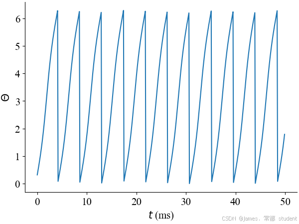
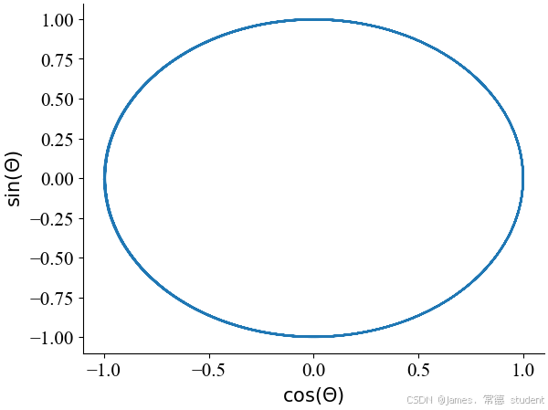
上述两张图均是在 θ \theta θ神经元在接收到强度为 6 的输入时的变化,其中左图展示了 θ \theta θ随时间的演化,右图展示了 sin ( θ ) \sin (\theta) sin(θ)和 cos ( θ ) \cos (\theta) cos(θ)的相图关系。
和 QIF 模型相比,经过推导和简化后的 θ \theta θ 神经元模型不再需要显式地重置发放脉冲的神经元,而是通过将 θ \theta θ 限制在 ( 0 , 2 π ) (0, 2\pi) (0,2π) 的区间上隐式地完成这一操作(如左图所示)。观察仿真过程中 ( sin θ , cos θ ) (\sin \theta, \cos \theta) (sinθ,cosθ) 的值,则可以将 θ \theta θ 在 ( 0 , 2 π ) (0, 2\pi) (0,2π) 的变化视作一个圆周运动,每当 θ \theta θ 到达 2 π 2\pi 2π 处,神经元便会被“重置”到 0 位置,从而使 θ \theta θ 的连续性不被破坏(如右图所示)。
5. QIF 模型的优点和不足
5.1. QIF 模型的优点
- 简洁性:QIF模型通过一个简单的二次方程来描述神经元的膜电位变化,相较于更复杂的Hodgkin-Huxley模型,其参数较少且计算量小得多。
- 计算效率:这使得它在大规模网络模拟中非常高效。
准确捕捉关键动力学特征 - 基本行为再现:尽管简化,QIF模型能够很好地再现神经元的基本行为,如阈值激发、放电频率适应性和尖峰后的复极化等现象。
- 尖峰生成过程:特别是它能较好地模拟接近阈值时的尖峰生成过程。
- 理论分析便利:对于某些情况下的QIF模型,可以得到解析解,这为理论分析提供了便利,并有助于理解神经元和神经网络的动力学特性。
- 参数调整:QIF模型可以通过调整参数来模拟不同类型的神经元行为,包括不同的放电模式和适应性特性。
- 扩展性:还可以扩展到包含噪声、突触输入等因素的复杂场景。
5.2. QIF 模型的不足
- 忽略生物物理细节:虽然QIF模型在描述基本的神经元动力学方面表现良好,但它忽略了大量生物物理细节,例如离子通道的具体类型及其动态变化。
- 应用限制:因此,在需要精确模拟特定离子电流或药物作用机制的研究中,它的应用受到限制。
- 复杂非线性现象:QIF模型虽然能捕捉到一些非线性特性,但对于一些复杂的非线性现象(如混沌放电模式)可能无法提供足够的描述能力。
- 异质化群体模拟:在处理高度异质化的神经元群体或复杂的突触连接时,QIF模型可能不够灵活。
- 特定神经元行为:对于某些特定类型的神经元(如那些表现出丰富多样的适应性特性的神经元),可能需要更复杂的模型来准确描述。
- 参数提取困难:由于QIF模型的高度抽象性,直接从实验数据中提取模型参数并进行验证可能会遇到困难。
- 实际应用限制:这在一定程度上限制了其在实际应用中的广泛采用。
6. 思考与总结
QIF模型作为一种平衡了简洁性和生物学现实性的工具,在神经科学研究中有其独特的优势,尤其是在大规模网络模拟和理论分析中。然而,它也存在一定的局限性,特别是在需要考虑详细生物物理机制或复杂动力学特性的情况下。选择使用哪种模型取决于具体的研究目标和需求。


 被折叠的 条评论
为什么被折叠?
被折叠的 条评论
为什么被折叠?
 到【灌水乐园】发言


