基于随机森林算法的信用风险评估项目-优快云博客

本文链接：https://blog.youkuaiyun.com/weixin_71288092/article/details/146966941

引言

这是一个基于随机森林算法的德国信用风险评估项目，主要目的是构建一个机器学习模型来评估德国客户的信用风险，判断客户是否为高风险客户。

# -*- coding: utf-8 -*-
"""
德国信用风险评估随机森林模型
"""
# 基础库导入
import pandas as pd
import numpy as np
import matplotlib.pyplot as plt
import seaborn as sns
from sklearn.model_selection import train_test_split, GridSearchCV
from sklearn.ensemble import RandomForestClassifier
from sklearn.metrics import (accuracy_score, confusion_matrix,
                             classification_report, roc_curve, auc)
from sklearn.preprocessing import LabelEncoder, MinMaxScaler

import os
os.environ["QT_QPA_PLATFORM_PLUGIN_PATH"] = ".venv\Lib\site-packages\PyQt5\Qt5\plugins"

plt.rcParams['font.sans-serif'] = ['SimHei']
# 解决负号显示为方块的问题
plt.rcParams['axes.unicode_minus'] = False
plt.style.use('ggplot')  # 设置绘图风格

# 数据加载与探索
url = "https://archive.ics.uci.edu/ml/machine-learning-databases/statlog/german/german.data"
columns = ['status', 'duration', 'credit_history', 'purpose', 'amount',
           'savings', 'employment', 'installment_rate', 'personal_status',
           'other_debtors', 'residence', 'property', 'age',
           'other_installments', 'housing', 'existing_credits',
           'job', 'dependents', 'telephone', 'foreign_worker', 'risk']

#df = pd.read_csv(url, delim_whitespace=True, names=columns)
df = pd.read_csv(url, sep='\s+', names=columns)
# 数据预处理
# 将目标变量转换为0/1（1表示高风险）
df['risk'] = df['risk'].map({1:0, 2:1})

# 类别型特征编码
categorical_features = ['status', 'credit_history', 'purpose', 'savings',
                        'employment', 'personal_status', 'other_debtors',
                        'property', 'other_installments', 'housing',
                        'job', 'telephone', 'foreign_worker']

label_encoders = {}
for col in categorical_features:
    le = LabelEncoder()
    df[col] = le.fit_transform(df[col])
    label_encoders[col] = le

# 数值型特征归一化
numerical_features = ['duration', 'amount', 'installment_rate', 'age',
                      'residence', 'existing_credits', 'dependents']
scaler = MinMaxScaler()
df[numerical_features] = scaler.fit_transform(df[numerical_features])

# 划分数据集
X = df.drop('risk', axis=1)
y = df['risk']
X_train, X_test, y_train, y_test = train_test_split(X, y, test_size=0.3,
                                                    random_state=42,
                                                    stratify=y)

# 随机森林模型训练
# 初始化基础模型
rf_base = RandomForestClassifier(random_state=42, class_weight='balanced')
rf_base.fit(X_train, y_train)

# 参数网格
param_grid = {
    'n_estimators': [100, 200],
    'max_depth': [5, 10, None],
    'min_samples_split': [2, 5],
    'max_features': ['sqrt', 0.8]
}

# 网格搜索优化
grid_search = GridSearchCV(rf_base, param_grid, cv=5, scoring='f1', n_jobs=-1)
grid_search.fit(X_train, y_train)

# 获取最优模型
best_rf = grid_search.best_estimator_



# 模型评估
# 测试集预测
y_pred = best_rf.predict(X_test)
y_proba = best_rf.predict_proba(X_test)[:, 1]

# 评估指标
print("="*40)
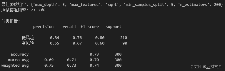
print("最佳参数组合:", grid_search.best_params_)
print("测试集准确率: {:.2f}%".format(accuracy_score(y_test, y_pred)*100))
print("\n分类报告:")
print(classification_report(y_test, y_pred, target_names=['低风险', '高风险']))




# 可视化部分
plt.style.use('ggplot')

# 特征重要性
feature_importance = pd.Series(best_rf.feature_importances_, index=X.columns)
top_features = feature_importance.sort_values(ascending=False).head(10)

plt.figure(figsize=(10,6))
top_features.sort_values().plot(kind='barh')
plt.title('Top 10 特征重要性')
plt.xlabel('重要性得分')
plt.ylabel('特征名称')
plt.tight_layout()
plt.show()



# 混淆矩阵
plt.figure(figsize=(6,6))
sns.heatmap(confusion_matrix(y_test, y_pred), 
            annot=True, fmt='d', cmap='Blues',
            xticklabels=['低风险', '高风险'],
            yticklabels=['低风险', '高风险'])
plt.title('混淆矩阵')
plt.ylabel('真实标签')
plt.xlabel('预测标签')
plt.show()




# ROC曲线
fpr, tpr, thresholds = roc_curve(y_test, y_proba)
roc_auc = auc(fpr, tpr)

plt.figure(figsize=(8,6))
plt.plot(fpr, tpr, color='darkorange', lw=2, 
         label='ROC曲线 (AUC = %0.2f)' % roc_auc)
plt.plot([0, 1], [0, 1], color='navy', lw=2, linestyle='--')
plt.xlim([0.0, 1.0])
plt.ylim([0.0, 1.05])
plt.xlabel('假正率')
plt.ylabel('真正率')
plt.title('受试者工作特征曲线')
plt.legend(loc="lower right")
plt.show()



# 风险客户特征分析（示例）
risk_df = df[df['risk'] == 1]

# 贷款目的分析
purpose_mapping = label_encoders['purpose'].classes_
plt.figure(figsize=(10,6))
sns.countplot(x='purpose', data=risk_df, order=risk_df['purpose'].value_counts().index)
plt.xticks(ticks=range(len(purpose_mapping)), labels=purpose_mapping, rotation=45)
plt.title('高风险客户贷款目的分布')
plt.xlabel('贷款目的')
plt.ylabel('数量')
plt.tight_layout()
plt.show()

# 存款情况分析
savings_mapping = label_encoders['savings'].classes_  # 获取存款情况的原始类别

# 定义颜色列表，可根据需要调整
colors = sns.color_palette('pastel')[:len(savings_mapping)]

# 定义爆炸效果，这里突出显示第一个部分，可根据需要调整
explode = [0.1] + [0] * (len(savings_mapping) - 1)

plt.figure(figsize=(8, 5))  # 设置图形大小
risk_df['savings'].value_counts().sort_index().plot(
    kind='pie',
    autopct='%1.1f%%',
    labels=savings_mapping,
    colors=colors,
    explode=explode,
    shadow=True,  # 添加阴影
    startangle=90  # 设置起始角度
)
plt.title('高风险客户储蓄账户分布', fontsize=14)  # 设置标题并调整字体大小
plt.axis('equal')  # 保证饼图是圆形
plt.tight_layout()  # 自动调整布局
plt.show()  # 显示图

总体介绍

1. 数据获取与处理

数据加载：从 https://archive.ics.uci.edu/ml/machine-learning-databases/statlog/german/german.data 下载德国信用风险数据集。
数据预处理：
- 将目标变量 risk 转换为 0/1 编码，其中 1 表示高风险。
- 对类别型特征使用 LabelEncoder 进行编码。
- 对数值型特征使用 MinMaxScaler 进行归一化处理。

2. 模型构建与训练

模型选择：使用随机森林分类器 RandomForestClassifier 作为预测模型。
模型优化：通过 GridSearchCV 进行网格搜索，寻找最优的模型参数组合，以提高模型性能。

3. 模型评估

预测结果：使用最优模型对测试集进行预测，得到预测标签 y_pred 和预测概率 y_proba。
评估指标：计算并输出最佳参数组合、测试集准确率、分类报告等评估指标。

4. 可视化分析

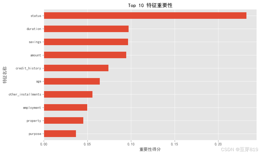
特征重要性：绘制前 10 个最重要特征的柱状图，帮助理解哪些特征对模型预测影响最大。
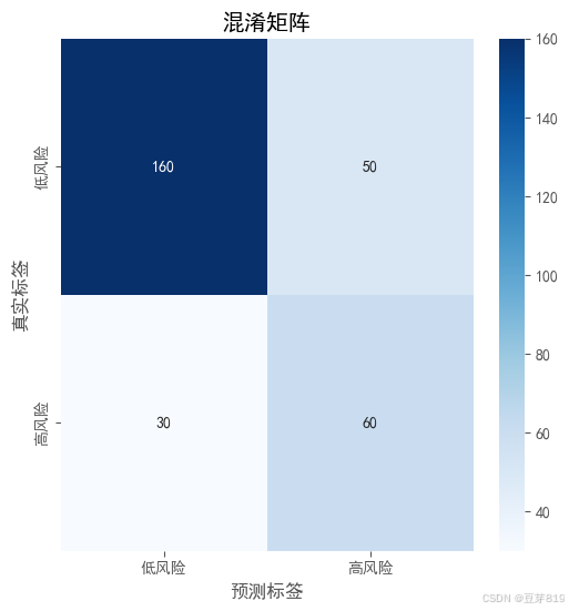
混淆矩阵：使用热力图展示模型在测试集上的分类结果，直观呈现模型的误判情况。
ROC 曲线：绘制受试者工作特征曲线，计算并展示曲线下面积（AUC），评估模型的分类性能。

5. 风险客户特征分析

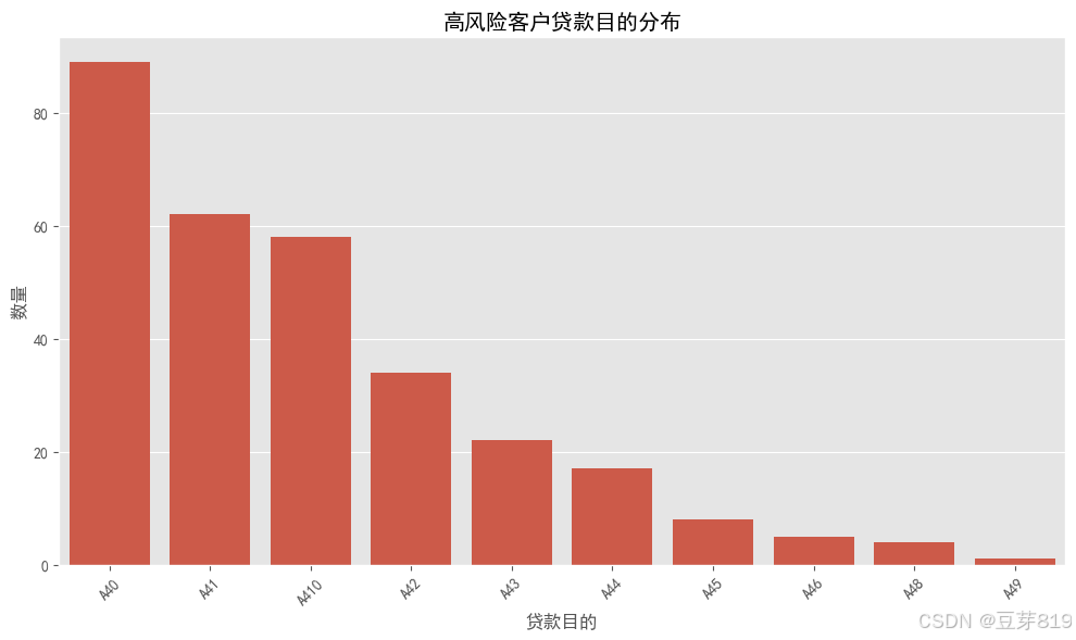
贷款目的分析：统计高风险客户的贷款目的分布，绘制柱状图展示不同贷款目的的客户数量。
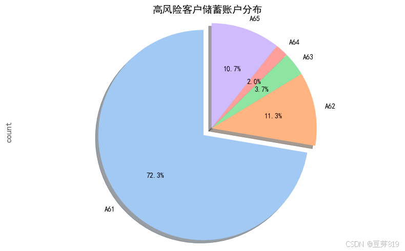
存款情况分析：统计高风险客户的存款账户分布，绘制饼图展示不同存款情况的客户占比。

模块分解

1. 导入库和设置环境变量

# -*- coding: utf-8 -*-
"""
德国信用风险评估随机森林模型
"""
# 基础库导入
import pandas as pd  # 用于数据处理和分析
import numpy as np  # 用于科学计算
import matplotlib.pyplot as plt  # 用于数据可视化
import seaborn as sns  # 基于matplotlib的高级可视化库
from sklearn.model_selection import train_test_split, GridSearchCV  # 用于划分数据集和网格搜索
from sklearn.ensemble import RandomForestClassifier  # 随机森林分类器
from sklearn.metrics import (accuracy_score, confusion_matrix,
                             classification_report, roc_curve, auc)  # 模型评估指标
from sklearn.preprocessing import LabelEncoder, MinMaxScaler  # 用于特征编码和归一化

import os
# 设置Qt平台插件路径，解决可视化窗口显示问题
os.environ["QT_QPA_PLATFORM_PLUGIN_PATH"] = "F:\cv\.venv\Lib\site-packages\PyQt5\Qt5\plugins"

plt.rcParams['font.sans-serif'] = ['SimHei']
# 解决负号显示为方块的问题
plt.rcParams['axes.unicode_minus'] = False
plt.style.use('ggplot')  # 设置绘图风格

pandas：用于数据处理和分析，提供了 DataFrame 和 Series 等数据结构，方便对表格数据进行操作。
numpy：用于科学计算，提供了高效的多维数组对象和各种数学函数。
matplotlib 和 seaborn：用于数据可视化，matplotlib 是基础的绘图库，seaborn 基于 matplotlib 提供了更高级、更美观的绘图接口。
sklearn 相关模块：
- train_test_split：用于将数据集划分为训练集和测试集。
- GridSearchCV：用于进行网格搜索，自动寻找模型的最优参数组合。
- RandomForestClassifier：随机森林分类器，是一种集成学习算法。
- accuracy_score、confusion_matrix、classification_report、roc_curve、auc：用于评估模型的性能。
- LabelEncoder：用于对类别型特征进行编码，将字符串类型的类别转换为数值类型。
- MinMaxScaler：用于对数值型特征进行归一化处理，将特征值缩放到 [0, 1] 区间。
os.environ["QT_QPA_PLATFORM_PLUGIN_PATH"]：设置 Qt 平台插件的路径，解决使用 matplotlib 显示图形时可能出现的 Qt 插件找不到的问题。

2. 数据加载与探索

# 数据加载与探索
url = "https://archive.ics.uci.edu/ml/machine-learning-databases/statlog/german/german.data"
columns = ['status', 'duration', 'credit_history', 'purpose', 'amount',
           'savings', 'employment', 'installment_rate', 'personal_status',
           'other_debtors', 'residence', 'property', 'age',
           'other_installments', 'housing', 'existing_credits',
           'job', 'dependents', 'telephone', 'foreign_worker', 'risk']

# 从指定URL读取数据，使用正则表达式 \s+ 作为分隔符
df = pd.read_csv(url, sep='\s+', names=columns)

url：指定数据集的网络地址，该数据集是德国信用风险评估的公开数据集。
columns：定义数据集中各列的名称。
pd.read_csv：从指定的 URL 读取数据，sep='\s+' 表示使用一个或多个空白字符作为分隔符，names=columns 表示使用 columns 列表中的名称作为列名。

3. 数据预处理

# 将目标变量转换为0/1（1表示高风险）
df['risk'] = df['risk'].map({1:0, 2:1})

# 类别型特征编码
categorical_features = ['status', 'credit_history', 'purpose', 'savings',
                        'employment', 'personal_status', 'other_debtors',
                        'property', 'other_installments', 'housing',
                        'job', 'telephone', 'foreign_worker']

label_encoders = {}
for col in categorical_features:
    le = LabelEncoder()  # 创建LabelEncoder对象
    df[col] = le.fit_transform(df[col])  # 对类别型特征进行编码
    label_encoders[col] = le  # 保存每个特征的编码器

# 数值型特征归一化
numerical_features = ['duration', 'amount', 'installment_rate', 'age',
                      'residence', 'existing_credits', 'dependents']
scaler = MinMaxScaler()  # 创建MinMaxScaler对象
df[numerical_features] = scaler.fit_transform(df[numerical_features])  # 对数值型特征进行归一化

map 方法：将 risk 列中的值 1 映射为 0，2 映射为 1，使得 1 表示高风险，0 表示低风险。

categorical_features：定义所有类别型特征的列名。
LabelEncoder：对每个类别型特征进行编码，将字符串类型的类别转换为连续的整数。
label_encoders：保存每个类别型特征对应的编码器，方便后续对新数据进行编码或者逆编码。
numerical_features：定义所有数值型特征的列名。
MinMaxScaler：对数值型特征进行归一化处理，将每个特征的取值范围缩放到 [0, 1] 之间。

4. 划分数据集

# 划分数据集
X = df.drop('risk', axis=1)  # 特征矩阵
y = df['risk']  # 目标变量
# 划分训练集和测试集，测试集占比30%，保持类别分布一致
X_train, X_test, y_train, y_test = train_test_split(X, y, test_size=0.3,
                                                    random_state=42,
                                                    stratify=y)

X = df.drop('risk', axis=1)：将除 risk 列之外的所有列作为特征矩阵 X。
y = df['risk']：将 risk 列作为目标变量 y。
train_test_split：将数据集划分为训练集和测试集，test_size=0.3 表示测试集占总数据集的 30%，random_state=42 用于设置随机种子，保证每次划分的结果相同，stratify=y 表示按照目标变量的类别分布进行分层抽样，确保训练集和测试集中各类别的比例与原始数据集相同。

5. 随机森林模型训练

# 初始化基础模型
rf_base = RandomForestClassifier(random_state=42, class_weight='balanced')  # 创建随机森林分类器，处理类别不平衡问题
rf_base.fit(X_train, y_train)  # 训练模型

# 参数网格
param_grid = {
    'n_estimators': [100, 200],  # 决策树的数量
    'max_depth': [5, 10, None],  # 决策树的最大深度
    'min_samples_split': [2, 5],  # 拆分内部节点所需的最小样本数
    'max_features': ['sqrt', 0.8]  # 寻找最佳分割时要考虑的特征数量
}

# 网格搜索优化
grid_search = GridSearchCV(rf_base, param_grid, cv=5, scoring='f1', n_jobs=-1)  # 创建网格搜索对象
grid_search.fit(X_train, y_train)  # 进行网格搜索

# 获取最优模型
best_rf = grid_search.best_estimator_  # 获取最优模型

RandomForestClassifier：初始化一个随机森林分类器，random_state=42 保证每次模型训练的结果可复现，class_weight='balanced' 用于处理类别不平衡问题，自动调整各类别的权重。
fit 方法：使用训练集数据对模型进行训练。
param_grid：定义需要搜索的参数组合，包括决策树的数量 n_estimators、决策树的最大深度 max_depth、拆分内部节点所需的最小样本数 min_samples_split 和寻找最佳分割时要考虑的特征数量 max_features。
GridSearchCV：创建一个网格搜索对象，cv=5 表示进行 5 折交叉验证，scoring='f1' 表示使用 F1 分数作为评估指标，n_jobs=-1 表示使用所有可用的 CPU 核心进行并行计算。
fit 方法：对训练集进行网格搜索，寻找最优的参数组合。
best_estimator_：获取网格搜索得到的最优模型。

6. 模型评估

# 测试集预测
y_pred = best_rf.predict(X_test)  # 预测标签
y_proba = best_rf.predict_proba(X_test)[:, 1]  # 预测概率

# 评估指标
print("="*40)
print("最佳参数组合:", grid_search.best_params_)  # 输出最优参数组合
print("测试集准确率: {:.2f}%".format(accuracy_score(y_test, y_pred)*100))  # 输出测试集准确率
print("\n分类报告:")
print(classification_report(y_test, y_pred, target_names=['低风险', '高风险']))  # 输出分类报告

predict 方法：使用最优模型对测试集进行预测，得到预测标签 y_pred。
predict_proba 方法：使用最优模型对测试集进行预测，得到每个样本属于各个类别的概率，[:, 1] 表示取属于高风险类别的概率。
accuracy_score：计算测试集的准确率。
classification_report：生成分类报告，包括精确率、召回率、F1 分数等评估指标。

7. 可视化部分

特征重要性

plt.style.use('ggplot')  # 设置绘图风格

# 特征重要性
feature_importance = pd.Series(best_rf.feature_importances_, index=X.columns)  # 计算特征重要性
top_features = feature_importance.sort_values(ascending=False).head(10)  # 选取前10个重要特征

plt.figure(figsize=(10,6))  # 设置图形大小
top_features.sort_values().plot(kind='barh')  # 绘制水平柱状图
plt.title('Top 10 特征重要性')  # 设置标题
plt.xlabel('重要性得分')  # 设置x轴标签
plt.ylabel('特征名称')  # 设置y轴标签
plt.tight_layout()  # 自动调整布局
plt.show()  # 显示图形

best_rf.feature_importances_：获取最优模型中每个特征的重要性得分。
pd.Series：将特征重要性得分转换为 Series 对象，方便后续处理。
sort_values：对特征重要性得分进行排序，选取前 10 个最重要的特征。
plot(kind='barh')：绘制水平柱状图，展示前 10 个特征的重要性得分。

混淆矩阵

plt.figure(figsize=(6,6))  # 设置图形大小
sns.heatmap(confusion_matrix(y_test, y_pred), 
            annot=True, fmt='d', cmap='Blues',  # 绘制热力图，显示数值
            xticklabels=['低风险', '高风险'],
            yticklabels=['低风险', '高风险'])
plt.title('混淆矩阵')  # 设置标题
plt.ylabel('真实标签')  # 设置y轴标签
plt.xlabel('预测标签')  # 设置x轴标签
plt.show()  # 显示图形

confusion_matrix：计算测试集的混淆矩阵。
sns.heatmap：使用 seaborn 库绘制热力图，直观展示模型的分类结果。

ROC曲线

fpr, tpr, thresholds = roc_curve(y_test, y_proba)  # 计算ROC曲线的假正率、真正率和阈值
roc_auc = auc(fpr, tpr)  # 计算ROC曲线下的面积

plt.figure(figsize=(8,6))  # 设置图形大小
plt.plot(fpr, tpr, color='darkorange', lw=2, 
         label='ROC曲线 (AUC = %0.2f)' % roc_auc)  # 绘制ROC曲线
plt.plot([0, 1], [0, 1], color='navy', lw=2, linestyle='--')  # 绘制随机分类器的对角线
plt.xlim([0.0, 1.0])  # 设置x轴范围
plt.ylim([0.0, 1.05])  # 设置y轴范围
plt.xlabel('假正率')  # 设置x轴标签
plt.ylabel('真正率')  # 设置y轴标签
plt.title('受试者工作特征曲线')  # 设置标题
plt.legend(loc="lower right")  # 设置图例位置
plt.show()  # 显示图形

roc_curve：计算 ROC 曲线的假正率 fpr、真正率 tpr 和阈值 thresholds。
auc：计算 ROC 曲线下的面积 roc_auc。
plt.plot：绘制 ROC 曲线和随机分类器的对角线。

8. 风险客户特征分析

贷款目的分析

# 风险客户特征分析（示例）
risk_df = df[df['risk'] == 1]  # 筛选出高风险客户

# 贷款目的分析
purpose_mapping = label_encoders['purpose'].classes_  # 获取贷款目的的原始类别
plt.figure(figsize=(10,6))  # 设置图形大小
sns.countplot(x='purpose', data=risk_df, order=risk_df['purpose'].value_counts().index)  # 绘制柱状图
plt.xticks(ticks=range(len(purpose_mapping)), labels=purpose_mapping, rotation=45)  # 设置x轴刻度和标签
plt.title('高风险客户贷款目的分布')  # 设置标题
plt.xlabel('贷款目的')  # 设置x轴标签
plt.ylabel('数量')  # 设置y轴标签
plt.tight_layout()  # 自动调整布局
plt.show()  # 显示图形

risk_df = df[df['risk'] == 1]：筛选出高风险客户的数据。
label_encoders['purpose'].classes_：获取 purpose 特征的原始类别。
sns.countplot：绘制柱状图，展示高风险客户的贷款目的分布。

存款情况分析

# 存款情况分析
savings_mapping = label_encoders['savings'].classes_  # 获取存款情况的原始类别

# 定义颜色列表，可根据需要调整
colors = sns.color_palette('pastel')[:len(savings_mapping)]

# 定义爆炸效果，这里突出显示第一个部分，可根据需要调整
explode = [0.1] + [0] * (len(savings_mapping) - 1)

plt.figure(figsize=(8, 5))  # 设置图形大小
risk_df['savings'].value_counts().sort_index().plot(
    kind='pie',
    autopct='%1.1f%%',
    labels=savings_mapping,
    colors=colors,
    explode=explode,
    shadow=True,  # 添加阴影
    startangle=90  # 设置起始角度
)
plt.title('高风险客户储蓄账户分布', fontsize=14)  # 设置标题并调整字体大小
plt.axis('equal')  # 保证饼图是圆形
plt.tight_layout()  # 自动调整布局
plt.show()  # 显示图