卷积神经网络算法笔记（1.LeNet-5）-优快云博客

本文详细介绍了如何使用经典的LeNet-5卷积神经网络对MNIST-Fashion数据集进行图像分类，包括网络结构、GPU加速、参数初始化、数据加载、损失函数和优化策略，以及训练过程中的性能评估和可视化。

摘要生成于 C知道，由 DeepSeek-R1 满血版支持，前往体验 >

摘要：本博文主要介绍使用卷积神经网络完成MNIST-Fashion数据集分类任务的算法过程。

0、背景介绍

MNIST-Fashion数据集：包含了10个不同种类的时尚商品的灰度图像。每个图像的尺寸为 $28×2828\times 28$ 像素。

这10个类别为：T恤/上衣（T-shirt/top）、裤子（Trouser）、毛衣（Pullover）、连衣裙（Dress）、外套（Coat）、凉鞋（Sandal）、衬衫（Shirt）、运动鞋（Sneaker）、包（Bag）和踝靴（Ankle boot）。
LeNet-5模型： 经典的卷积神经网络（CNN），由Yann LeCun等人于1998年提出。这一发明非常超前，跨越了传统视觉算法的思路，历史性的提出了“卷积”的思想用于图像特征的提取。LeNet-5模型由7个层组成，包括3个卷积层、2个池化层和2个全连接层。

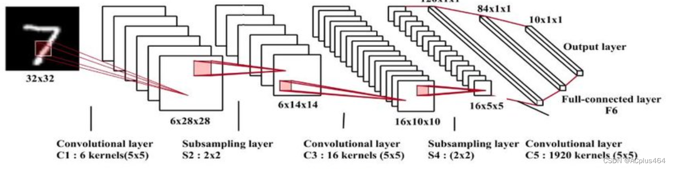
下面是LeNet-5模型的层次结构：
- 第一层（卷积层）：输入是 $32×3232\times32$ 的灰度图像。使用6个 $5×55\times5$ 的卷积核对输入进行卷积操作，得到6个特征图。每个特征图的大小为 $28×2828\times 28$ 。
- 第二层（池化层）：对每个特征图进行 $2×22\times 2$ 的均值池化操作，将特征图的尺寸减半，得到6个 $14×1414\times 14$ 的特征图。
- 第三层（卷积层）：使用16个 $5×55\times 5$ 的卷积核对第二层的特征图进行卷积操作，得到16个 $10×1010\times 10$ 的特征图。
- 第四层（池化层）：对每个特征图进行 $2×22\times 2$ 的平均池化操作，将特征图的尺寸减半，得到16个 $5×55\times 5$ 的特征图。
- 第五层（全连接层）：将第四层的特征图展平为一个向量，并与120个神经元进行全连接。
- 第六层（全连接层）：与84个神经元进行全连接。
- 第七层（输出层）：使用softmax激活函数将84个神经元的输出映射为10个类别的概率分布，表示输入图像属于每个类别的概率。

1、网络定义

根据上文的描述，我们使用nn.Sequential()方法，一层一层地堆叠7层网络的结构即可：

class Reshape(nn.Module):
    def forward(self, x):
        x = x.view(-1, 1, 28, 28)
        return x
    
net = nn.Sequential(
    Reshape(),
    nn.Conv2d(1, 6, kernel_size=5, padding=2), nn.Sigmoid(),
    nn.AvgPool2d(2, stride=2),
    nn.Conv2d(6, 16, kernel_size=5), nn.Sigmoid(),
    nn.AvgPool2d(2, stride=2), nn.Flatten(),
    nn.Linear(16 * 5 * 5, 120), nn.Sigmoid(),
    nn.Linear(120, 84), nn.Sigmoid(),
    nn.Linear(84, 10),
)

2、使用GPU

使用GPU进行训练和测试的加速。思路如下：

配置device
将net迁移到device上
将训练数据和测试（验证）数据迁移到device上

device = torch.device("cuda" if torch.cuda.is_available() else "cpu")
net.to(device)

3、网络参数初始化

此处使用了nn.apply()方法，对nn.Sequential()搭建的网络进行参数初始化。后续的网络很多也沿用了这一方法：

def weights_init(layer):
    if isinstance(layer, nn.Conv2d) or isinstance(layer, nn.Linear):
        nn.init.xavier_uniform_(layer.weight)
        nn.init.zeros_(layer.bias)
        
net.apply(weights_init)

4、数据加载

使用d2l算法库，直接拉取数据集即可，这样非常简单，不用自己下载和保存：

batch_size = 128
train_iter, test_iter = d2l.load_data_fashion_mnist(batch_size=batch_size)

两行代码就能搞定。这样返回的train_iter, test_iter是迭代器函数，每调用一次返回一个批次的数据。

5、损失函数与优化器

使用CrossEntropy损失函数和随机梯度下降（SGD）算法：

loss = nn.CrossEntropyLoss()
optimizer = torch.optim.SGD(net.parameters(), lr=0.9)

6、训练

对于图像分类任务，除了要定义损失函数外，还要定义精度（acc，accuracy）函数：

def calculate_accuracy(trues, preds):
    total_samples = len(trues)
    correct_predictions = sum(1 for true, pred in zip(trues, preds) if true == pred)
    accuracy = correct_predictions / total_samples
    return accuracy

下面开始训练：

epochs = 20
lr = 0.05

train_err_list = [] # loss列表，画图用
train_acc_list = []
test_err_list = [] # acc列表，画图用
test_acc_list = []
start_time = time.time()
for epoch in range(epochs):
    epoch_start_time = time.time()
    train_err = 0
    net.train() # 一些深度模型可能需要手动开启，之前那些小模型如线性回归模型可能就不需要？
    for batch_X, batch_Y in train_iter:
        # batch_X = batch_X.float()
        # batch_Y = batch_Y.float()
        # print(batch_X)
        
        batch_X = batch_X.to(device)
        batch_Y = batch_Y.to(device)
#         print(type(batch_X))
        
        # 前向传播
        outputs = net(batch_X) # torch.Size([256, 10])
#         print(outputs)
#         print(outputs.shape)
#         print(batch_Y.shape)
        loss_val = loss(outputs, batch_Y)

        # 反向传播和优化
        optimizer = torch.optim.SGD(net.parameters(), lr=lr)
        optimizer.zero_grad()
        loss_val.backward()
        optimizer.step()
        
        # 记录训练损失
        train_err_list.append(loss_val.item())
        
        # 计算训练Acc，记录
        trues = d2l.get_fashion_mnist_labels(batch_Y)
        preds = d2l.get_fashion_mnist_labels(outputs.argmax(axis=1))
        train_acc = calculate_accuracy(trues, preds)
        train_acc_list.append(train_acc)
        
       
    # 进行测试
    with torch.no_grad():
        for test_X, test_Y in test_iter:
            # 测试数据的迁移
            test_X = test_X.to(device)
            test_Y = test_Y.to(device)
            
            # 计算测试输出和测试loss
            test_outputs = net(test_X)
            test_err = loss(test_outputs, test_Y) # torch.sum(test_outputs != test_Y).item() / test_Y.shape[0]
            
            # 计算测试acc
            trues = d2l.get_fashion_mnist_labels(test_Y)
            preds = d2l.get_fashion_mnist_labels(net(test_X).argmax(axis=1))
            test_acc = calculate_accuracy(trues, preds)
            
            # 记录测试loss和测试acc
            print(f'At epoch {epoch+1}: train_acc {train_acc:.8f}, test_acc {test_acc}')
            test_err_list.append(test_err.item())
            test_acc_list.append(test_acc)
            break
            
    epoch_end_time = time.time()
    print(f"{device} time At epoch {epoch+1}: {epoch_end_time - epoch_start_time}")
    

end_time = time.time()
print(f"{device} time: {end_time - start_time}")

输出：

At epoch 1: train_acc 0.09166667, test_acc 0.105625
cuda time At epoch 1: 33.74168109893799
At epoch 2: train_acc 0.51250000, test_acc 0.54375
cuda time At epoch 2: 32.65597414970398
At epoch 3: train_acc 0.66458333, test_acc 0.675
cuda time At epoch 3: 32.79549026489258
At epoch 4: train_acc 0.88541667, test_acc 0.759375
cuda time At epoch 4: 33.176368951797485
At epoch 5: train_acc 0.82416667, test_acc 0.7828125
cuda time At epoch 5: 33.19402623176575
At epoch 6: train_acc 0.83583333, test_acc 0.775
cuda time At epoch 6: 32.876006841659546
At epoch 7: train_acc 0.83666667, test_acc 0.790625
cuda time At epoch 7: 33.013068437576294
At epoch 8: train_acc 0.83583333, test_acc 0.815
cuda time At epoch 8: 32.882542848587036
At epoch 9: train_acc 0.85833333, test_acc 0.8271875
cuda time At epoch 9: 32.794219970703125
At epoch 10: train_acc 0.88750000, test_acc 0.8328125
cuda time At epoch 10: 32.84580612182617

绘制训练和测试过程中损失和精度的变化曲线：

# print(train_err_list)
# 绘制4个子图
plt.figure(figsize=(8, 6))

# 训练损失子图
plt.subplot(2, 2, 1)
plt.plot(train_err_list)
plt.title('Train Loss VS batch')

# 训练准确率子图
plt.subplot(2, 2, 2)
plt.plot(train_acc_list)
plt.title('Train Accuracy VS batch')

# 测试损失子图
plt.subplot(2, 2, 3)
plt.plot(test_err_list)
plt.title('Test Loss VS epoch')

# 测试准确率子图
plt.subplot(2, 2, 4)
plt.plot(test_acc_list)
plt.title('Test Accuracy VS epoch')

# 调整子图之间的间距
plt.tight_layout()

# 显示图形
plt.show()

7、预测

对于测试数据集，随机选取5个进行预测输出。（此处不展示效果）

def predict(net, test_iter, n=5):
    for X, y in test_iter:
        X, y = X.to(device), y.to(device)
        break
    trues = d2l.get_fashion_mnist_labels(y)
    preds = d2l.get_fashion_mnist_labels(net(X).argmax(axis=1))
    # print(trues)
    # print(preds)
    titles = [true + '\n' + pred for true, pred in zip(trues, preds)]
    d2l.show_images(X[0:n].reshape((n,28,28)), 1, n, titles=titles[0:n])
    
predict(net, test_iter)