


 本文介绍了监督学习的基本概念,包括分类与回归的区别,以鸢尾花和wave数据集为例展示了K近邻算法的应用。后续探讨了线性模型(如线性回归、岭回归和Lasso)在回归和分类中的原理与实战,以及它们在不同数据集上的性能优化。
文章目录
前言
监督学习
提示:这里可以添加本文要记录的大概内容:
例如:随着人工智能的不断发展,机器学习这门技术也越来越重要,很多人都开启了学习机器学习,本文就介绍了机器学习的基础内容。
提示:以下是本篇文章正文内容,下面案例可供参考
一、监督学习
1.分类与回归
分类问题:预测类别标签,这些标签来自预定义的可选列表
回归问题:预测一个连续值
区分以上两个任务的方法:输出是否具有某种连续性
1.鸢尾花分类
import numpy as np
import matplotlib.pyplot as plt
import pandas as pd
import mglearn
# 花的数据集在scikit-learn的datasets模块中
from sklearn.datasets import load_iris
iris_datasets = load_iris()
# load_iris返回的iris对象是一个bunch对象和字典非常相似,里面包含键和值
# 数据集中对应的键值对
print("keys\n{}".format(iris_datasets.keys()))
# 数据集中的数据
print(iris_datasets['data'])
# 测量过的每朵花的品种 数组
print(iris_datasets['target'])
print(iris_datasets['frame'])
# 对应种类的名称
print(iris_datasets['target_names'])
# 对应的值是数据集的简要说明
print(iris_datasets['DESCR'])
# 特征的名称:花瓣的长度和宽度,花萼的长度和宽度
print("x{}".format(iris_datasets['feature_names']))
# 文件的名称
print(iris_datasets['filename'])
# 数据集的模块
print(iris_datasets['data_module'])
# 使用train_test_split划分训练集和测试集
# 该函数将75%数据和对应标签作为训练数据,25%作为测试数据
# 利用伪随机数生成器将数据打乱
# 为确保多次运行的函数能够得到相同的结果,利用randon_state参数指定随机数生成的种子
from sklearn.model_selection import train_test_split
x_trian, x_test, y_train, y_test = train_test_split(
iris_datasets['data'], iris_datasets['target'], random_state=0
)
# 查看数据大小
print("x_train shape{}".format(x_trian.shape))
print("x_test shape{}".format(x_test.shape))
print("y_train shape{}".format(y_train.shape))
print("y_test shape{}".format(y_test.shape))
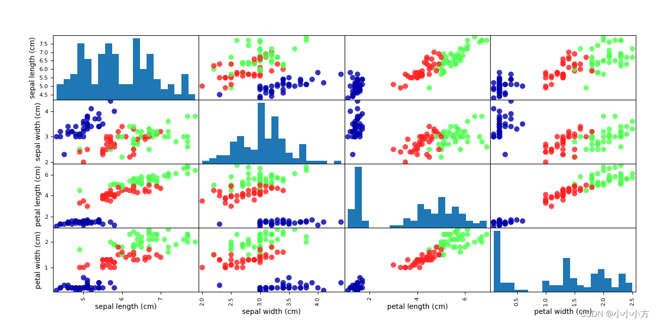
# 利用散点图矩阵检查数据的异常值和特殊值
# 散点矩阵图无法同时显示所有特征之间的关系
# 利用x_train中的数据创建dataframe,利用feature_names中的字符串对数据列进行标记
iris_dataframe = pd.DataFrame(x_trian, columns=iris_datasets.feature_names)
# 利用dataframe创建散点图矩阵,按y_train着色
grr = pd.plotting.scatter_matrix(iris_dataframe, c=y_train, figsize=(15, 15), marker='o', hist_kwds={'bins': 20}, s=60,
alpha=.8, cmap=mglearn.cm3)
# 展示散点图矩阵
plt.show()
运行结果:
keys
dict_keys(['data', 'target', 'frame', 'target_names', 'DESCR', 'feature_names', 'filename', 'data_module'])
[[5.1 3.5 1.4 0.2]
[4.9 3. 1.4 0.2]
[4.7 3.2 1.3 0.2]
[4.6 3.1 1.5 0.2]
[5. 3.6 1.4 0.2]
[5.4 3.9 1.7 0.4]
[4.6 3.4 1.4 0.3]
[5. 3.4 1.5 0.2]
[4.4 2.9 1.4 0.2]
[4.9 3.1 1.5 0.1]
[5.4 3.7 1.5 0.2]
[4.8 3.4 1.6 0.2]
[4.8 3. 1.4 0.1]
[4.3 3. 1.1 0.1]
[5.8 4. 1.2 0.2]
[5.7 4.4 1.5 0.4]
[5.4 3.9 1.3 0.4]
[5.1 3.5 1.4 0.3]
[5.7 3.8 1.7 0.3]
[5.1 3.8 1.5 0.3]
[5.4 3.4 1.7 0.2]
[5.1 3.7 1.5 0.4]
[4.6 3.6 1. 0.2]
[5.1 3.3 1.7 0.5]
[4.8 3.4 1.9 0.2]
[5. 3. 1.6 0.2]
[5. 3.4 1.6 0.4]
[5.2 3.5 1.5 0.2]
[5.2 3.4 1.4 0.2]
[4.7 3.2 1.6 0.2]
[4.8 3.1 1.6 0.2]
[5.4 3.4 1.5 0.4]
[5.2 4.1 1.5 0.1]
[5.5 4.2 1.4 0.2]
[4.9 3.1 1.5 0.2]
[5. 3.2 1.2 0.2]
[5.5 3.5 1.3 0.2]
[4.9 3.6 1.4 0.1]
[4.4 3. 1.3 0.2]
[5.1 3.4 1.5 0.2]
[5. 3.5 1.3 0.3]
[4.5 2.3 1.3 0.3]
[4.4 3.2 1.3 0.2]
[5. 3.5 1.6 0.6]
[5.1 3.8 1.9 0.4]
[4.8 3. 1.4 0.3]
[5.1 3.8 1.6 0.2]
[4.6 3.2 1.4 0.2]
[5.3 3.7 1.5 0.2]
[5. 3.3 1.4 0.2]
[7. 3.2 4.7 1.4]
[6.4 3.2 4.5 1.5]
[6.9 3.1 4.9 1.5]
[5.5 2.3 4. 1.3]
[6.5 2.8 4.6 1.5]
[5.7 2.8 4.5 1.3]
[6.3 3.3 4.7 1.6]
[4.9 2.4 3.3 1. ]
[6.6 2.9 4.6 1.3]
[5.2 2.7 3.9 1.4]
[5. 2. 3.5 1. ]
[5.9 3. 4.2 1.5]
[6. 2.2 4. 1. ]
[6.1 2.9 4.7 1.4]
[5.6 2.9 3.6 1.3]
[6.7 3.1 4.4 1.4]
[5.6 3. 4.5 1.5]
[5.8 2.7 4.1 1. ]
[6.2 2.2 4.5 1.5]
[5.6 2.5 3.9 1.1]
[5.9 3.2 4.8 1.8]
[6.1 2.8 4. 1.3]
[6.3 2.5 4.9 1.5]
[6.1 2.8 4.7 1.2]
[6.4 2.9 4.3 1.3]
[6.6 3. 4.4 1.4]
[6.8 2.8 4.8 1.4]
[6.7 3. 5. 1.7]
[6. 2.9 4.5 1.5]
[5.7 2.6 3.5 1. ]
[5.5 2.4 3.8 1.1]
[5.5 2.4 3.7 1. ]
[5.8 2.7 3.9 1.2]
[6. 2.7 5.1 1.6]
[5.4 3. 4.5 1.5]
[6. 3.4 4.5 1.6]
[6.7 3.1 4.7 1.5]
[6.3 2.3 4.4 1.3]
[5.6 3. 4.1 1.3]
[5.5 2.5 4. 1.3]
[5.5 2.6 4.4 1.2]
[6.1 3. 4.6 1.4]
[5.8 2.6 4. 1.2]
[5. 2.3 3.3 1. ]
[5.6 2.7 4.2 1.3]
[5.7 3. 4.2 1.2]
[5.7 2.9 4.2 1.3]
[6.2 2.9 4.3 1.3]
[5.1 2.5 3. 1.1]
[5.7 2.8 4.1 1.3]
[6.3 3.3 6. 2.5]
[5.8 2.7 5.1 1.9]
[7.1 3. 5.9 2.1]
[6.3 2.9 5.6 1.8]
[6.5 3. 5.8 2.2]
[7.6 3. 6.6 2.1]
[4.9 2.5 4.5 1.7]
[7.3 2.9 6.3 1.8]
[6.7 2.5 5.8 1.8]
[7.2 3.6 6.1 2.5]
[6.5 3.2 5.1 2. ]
[6.4 2.7 5.3 1.9]
[6.8 3. 5.5 2.1]
[5.7 2.5 5. 2. ]
[5.8 2.8 5.1 2.4]
[6.4 3.2 5.3 2.3]
[6.5 3. 5.5 1.8]
[7.7 3.8 6.7 2.2]
[7.7 2.6 6.9 2.3]
[6. 2.2 5. 1.5]
[6.9 3.2 5.7 2.3]
[5.6 2.8 4.9 2. ]
[7.7 2.8 6.7 2. ]
[6.3 2.7 4.9 1.8]
[6.7 3.3 5.7 2.1]
[7.2 3.2 6. 1.8]
[6.2 2.8 4.8 1.8]
[6.1 3. 4.9 1.8]
[6.4 2.8 5.6 2.1]
[7.2 3. 5.8 1.6]
[7.4 2.8 6.1 1.9]
[7.9 3.8 6.4 2. ]
[6.4 2.8 5.6 2.2]
[6.3 2.8 5.1 1.5]
[6.1 2.6 5.6 1.4]
[7.7 3. 6.1 2.3]
[6.3 3.4 5.6 2.4]
[6.4 3.1 5.5 1.8]
[6. 3. 4.8 1.8]
[6.9 3.1 5.4 2.1]
[6.7 3.1 5.6 2.4]
[6.9 3.1 5.1 2.3]
[5.8 2.7 5.1 1.9]
[6.8 3.2 5.9 2.3]
[6.7 3.3 5.7 2.5]
[6.7 3. 5.2 2.3]
[6.3 2.5 5. 1.9]
[6.5 3. 5.2 2. ]
[6.2 3.4 5.4 2.3]
[5.9 3. 5.1 1.8]]
[0 0 0 0 0 0 0 0 0 0 0 0 0 0 0 0 0 0 0 0 0 0 0 0 0 0 0 0 0 0 0 0 0 0 0 0 0
0 0 0 0 0 0 0 0 0 0 0 0 0 1 1 1 1 1 1 1 1 1 1 1 1 1 1 1 1 1 1 1 1 1 1 1 1
1 1 1 1 1 1 1 1 1 1 1 1 1 1 1 1 1 1 1 1 1 1 1 1 1 1 2 2 2 2 2 2 2 2 2 2 2
2 2 2 2 2 2 2 2 2 2 2 2 2 2 2 2 2 2 2 2 2 2 2 2 2 2 2 2 2 2 2 2 2 2 2 2 2
2 2]
None
['setosa' 'versicolor' 'virginica']
.. _iris_dataset:
Iris plants dataset
--------------------
**Data Set Characteristics:**
:Number of Instances: 150 (50 in each of three classes)
:Number of Attributes: 4 numeric, predictive attributes and the class
:Attribute Information:
- sepal length in cm
- sepal width in cm
- petal length in cm
- petal width in cm
- class:
- Iris-Setosa
- Iris-Versicolour
- Iris-Virginica
:Summary Statistics:
============== ==== ==== ======= ===== ====================
Min Max Mean SD Class Correlation
============== ==== ==== ======= ===== ====================
sepal length: 4.3 7.9 5.84 0.83 0.7826
sepal width: 2.0 4.4 3.05 0.43 -0.4194
petal length: 1.0 6.9 3.76 1.76 0.9490 (high!)
petal width: 0.1 2.5 1.20 0.76 0.9565 (high!)
============== ==== ==== ======= ===== ====================
:Missing Attribute Values: None
:Class Distribution: 33.3% for each of 3 classes.
:Creator: R.A. Fisher
:Donor: Michael Marshall (MARSHALL%PLU@io.arc.nasa.gov)
:Date: July, 1988
The famous Iris database, first used by Sir R.A. Fisher. The dataset is taken
from Fisher's paper. Note that it's the same as in R, but not as in the UCI
Machine Learning Repository, which has two wrong data points.
This is perhaps the best known database to be found in the
pattern recognition literature. Fisher's paper is a classic in the field and
is referenced frequently to this day. (See Duda & Hart, for example.) The
data set contains 3 classes of 50 instances each, where each class refers to a
type of iris plant. One class is linearly separable from the other 2; the
latter are NOT linearly separable from each other.
.. topic:: References
- Fisher, R.A. "The use of multiple measurements in taxonomic problems"
Annual Eugenics, 7, Part II, 179-188 (1936); also in "Contributions to
Mathematical Statistics" (John Wiley, NY, 1950).
- Duda, R.O., & Hart, P.E. (1973) Pattern Classification and Scene Analysis.
(Q327.D83) John Wiley & Sons. ISBN 0-471-22361-1. See page 218.
- Dasarathy, B.V. (1980) "Nosing Around the Neighborhood: A New System
Structure and Classification Rule for Recognition in Partially Exposed
Environments". IEEE Transactions on Pattern Analysis and Machine
Intelligence, Vol. PAMI-2, No. 1, 67-71.
- Gates, G.W. (1972) "The Reduced Nearest Neighbor Rule". IEEE Transactions
on Information Theory, May 1972, 431-433.
- See also: 1988 MLC Proceedings, 54-64. Cheeseman et al"s AUTOCLASS II
conceptual clustering system finds 3 classes in the data.
- Many, many more ...
x['sepal length (cm)', 'sepal width (cm)', 'petal length (cm)', 'petal width (cm)']
iris.csv
sklearn.datasets.data
x_train shape(112, 4)
x_test shape(38, 4)
y_train shape(112,)
y_test shape(38,)
2.构建第一个模型:k近邻算法
考虑训练集中与新数据最近的任意k个邻居,用这些邻居最多的类别做出预测。
scikit-learn 中所有的机器学习模型都在各自的类中实现,这些类被称为 Estimator
类。k 近邻分类算法是在 neighbors 模块的 KNeighborsClassifier 类中实现的。我们需
要将这个类实例化为一个对象,然后才能使用这个模型。这时我们需要设置模型的参数。
KNeighborsClassifier 最重要的参数就是邻居的数目,这里我们设为 1:
#fit方法基于训练数据构建模型
from sklearn.neighbors import KNeighborsClassifier
knn = KNeighborsClassifier(n_neighbors=1)
knn.fit(x_trian,y_train)

# 预测一个新的数据 转换成二维数组
x_new = np.array([[5,2.9,1,0.2]])
prediction = knn.predict(x_new)
print("prediction{}".format(prediction))
print("prediction target name{}".format(iris_datasets['target_names'][prediction]))

# 构建评估模型
y_pred = knn.predict(x_test)
print("test set prediction{}".format(y_pred))

# 计算测试集精度的2种方法
print("test set score:{:0.2f}".format(np.mean(y_test == y_pred)))
print("test set score:{:0.2f}".format(knn.score(x_test,y_test)))

运行结果:
prediction[0]
prediction target name['setosa']
test set prediction[2 1 0 2 0 2 0 1 1 1 2 1 1 1 1 0 1 1 0 0 2 1 0 0 2 0 0 1 1 0 2 1 0 2 2 1 0
 2]
test set score:0.97
test set score:0.97
2.泛化,过拟合欠拟合
一个模型能够对没见过的数据做出准确的预测,则称为能够从训练集泛化到测试集
过拟合:在拟合模型时,过分关注训练集的细节,得到了一个在训练集上表现很好但不能泛化到新数据上的模型。
欠拟合:无法抓住数据的全部内容以及数据中的变化,模型甚至在训练集上的表现都很差。
需要找到两者之间的一个最佳位置,可以得到最好的泛化能力。
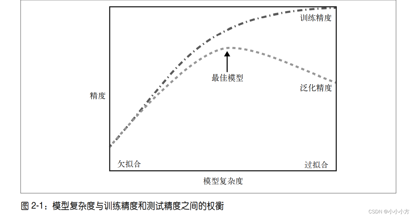
模型复杂度与训练数据集中的输入的变化密切相关:数据集中包含的数据点的变化范围越大,可以使用更复杂的模型,收集更多的数据,适当建立更复杂的模型。
3.监督学习算法
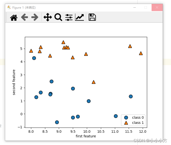
1.一些样本数据集
模拟二分类数据集:forge数据集,两个特征
import numpy as np
import matplotlib.pyplot as plt
import pandas as pd
import mglearn

# 1.生成二分类数据集forge数据集
x, y = mglearn.datasets.make_forge()
# 数据集绘图
mglearn.discrete_scatter(x[:, 0], x[:, 1], y)
plt.legend(["class 0", "class 1"], loc=4)
plt.xlabel("first feature")
plt.ylabel("second feature")
plt.show()
print("x.shape:{}".format(x.shape)

运行结果:
x.shape:(26, 2)
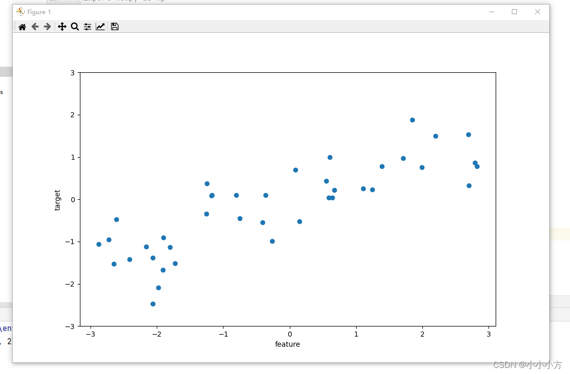
2.模拟回归算法的wave数据集
只有一个输入特征和一个连续的目标变量
plot()函数绘制二维线图
ylim()获取y轴的范围
# 2.生成回归算法wave数据集
x, y = mglearn.datasets.make_wave(n_samples=40)
# 参数o表示实心圆点标记
plt.plot(x, y, 'o')
plt.ylim(-3, 3)
plt.xlabel("feature")
plt.ylabel("target")
plt.show()
乳腺癌数据集,基于人体组织的测量数据来学习预测肿瘤是否为恶性
596个数据点,每个数据点30个特征,212个被标记为恶性,357个被标记为良性。
from sklearn.datasets import load_breast_cancer
cancer = load_breast_cancer()
print("cancer.keys():{}".format(cancer.keys()))
print("shape of cancer data:{}".format(cancer.data.shape))
print("sample counts per class:\n{}".format(
    {n:v for n,v in zip(cancer.target_names,np.bincount(cancer.target))}
))
print("feature name:{}".format(cancer.feature_names))

运行结果:
cancer.keys():dict_keys(['data', 'target', 'frame', 'target_names', 'DESCR', 'feature_names', 'filename', 'data_module'])
shape of cancer data:(569, 30)
sample counts per class:
{'malignant': 212, 'benign': 357}
feature name:['mean radius' 'mean texture' 'mean perimeter' 'mean area'
 'mean smoothness' 'mean compactness' 'mean concavity'
 'mean concave points' 'mean symmetry' 'mean fractal dimension'
 'radius error' 'texture error' 'perimeter error' 'area error'
 'smoothness error' 'compactness error' 'concavity error'
 'concave points error' 'symmetry error' 'fractal dimension error'
 'worst radius' 'worst texture' 'worst perimeter' 'worst area'
 'worst smoothness' 'worst compactness' 'worst concavity'
 'worst concave points' 'worst symmetry' 'worst fractal dimension']
波士顿房价数据集
506个数据,13个特征,但需要对找个数据集进行扩展,使得输入特征不止包含这13个测量结果,还要包含这些特征之间的乘积。
from sklearn.datasets import load_boston
boston = load_boston()
print("data shape:{}".format(boston.data.shape))
# 包含导出特征的方法叫做特征工程
x,y = mglearn.datasets.load_extended_boston()
# 最初的13个加上13个特征的两两组合得到91个特征
print("x.shape{}".format(x.shape))

运行结果:
data shape:(506, 13)
x.shape(506, 104)
2.K近邻
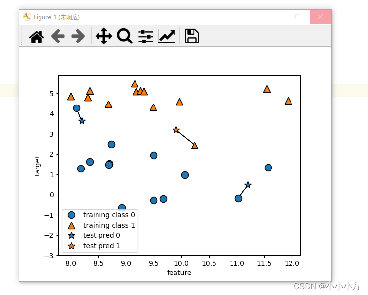
最简单的机器学习算法,给出这种分类算法在forge数据集上的应用。
mglearn.plots.plot_knn_classification(n_neighbors=1)
plt.show()

def plot_knn_classification(n_neighbors=1):
    X, y = make_forge()
    # 3个测试数据集
    X_test = np.array([[8.2, 3.66214339], [9.9, 3.2], [11.2, .5]])
    # 两点之间的欧几里得距离
    dist = euclidean_distances(X, X_test)
    # 返回的是元素值从小到大排序后的索引值的数组 0按行进行排序
    closest = np.argsort(dist, axis=0)

    for x, neighbors in zip(X_test, closest.T):
        # arrow箭头函数
        for neighbor in neighbors[:n_neighbors]:
            plt.arrow(x[0], x[1], X[neighbor, 0] - x[0],
                      X[neighbor, 1] - x[1], head_width=0, fc='k', ec='k')
    # 训练模型
    clf = KNeighborsClassifier(n_neighbors=n_neighbors).fit(X, y)
    # 绘制测试点
    test_points = discrete_scatter(X_test[:, 0], X_test[:, 1], clf.predict(X_test), markers="*")
    training_points = discrete_scatter(X[:, 0], X[:, 1], y)
    plt.legend(training_points + test_points, ["training class 0", "training class 1",
                                               "test pred 0", "test pred 1"])
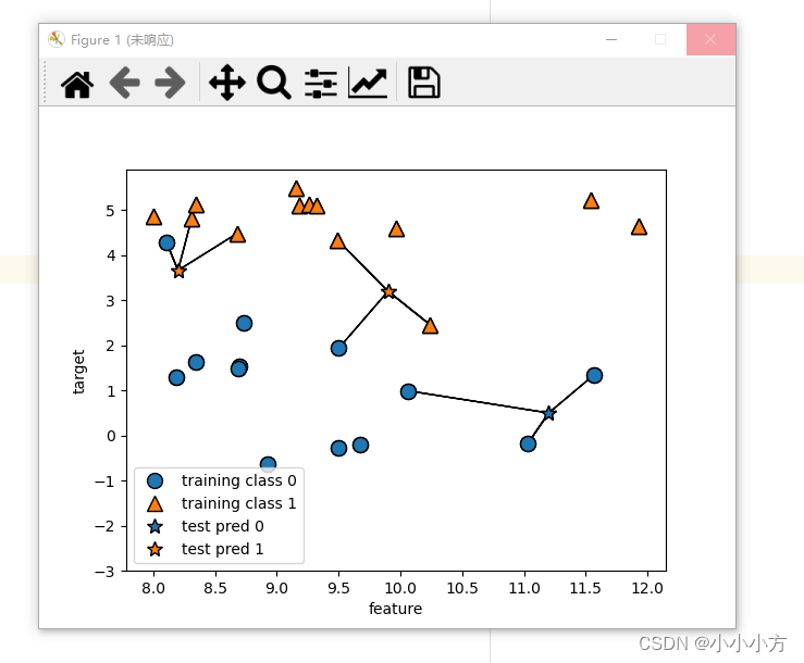
当考虑多个邻居的情况时,使用投票法来指定标签
mglearn.plots.plot_knn_classification(n_neighbors=3)
plt.show()
通过scikit-learn来引用k近邻算法,将数据分为训练集和测试集,评估模型的泛化能力。
import numpy as np
import matplotlib.pyplot as plt
import pandas as pd
import mglearn
# 通过scilit-learn来应用k近邻算法
from sklearn.model_selection import train_test_split
x,y = mglearn.datasets.make_forge()
x_train,x_test,y_train,y_test = train_test_split(x,y,random_state=0)
# 导入类并将其实例化
from sklearn.neighbors import KNeighborsClassifier
clf = KNeighborsClassifier(n_neighbors=3)
# 利用训练集进行拟合
clf.fit(x_train,y_train)
# 对测试集进行预测,对于每个数据点,都要计算他在训练集中最近邻,然后找出其中出现次数最多的类别
print("test set predictions:{}".format(clf.predict(x_test)))
# 评估模型泛化的能力
print("test set accuracy:{:.2f}".format(clf.score(x_test,y_test)))

运行结果:
test set predictions:[1 0 1 0 1 0 0]
test set accuracy:0.86
对于二维数据集,我们可以在xy平面上画出所有可能的测试结果,查看决策边界。
下列代码分别将 1 个、3 个和 9 个邻居三种情况的决策边界可视化
# 将1个,3个,9个邻居三种情况的决策边界可视化
fig,axes = plt.subplots(1,3,figsize=(10,3))
for n_neighbors,ax in zip([1,3,9],axes):
    # fit方法返回对象本身,所以我们可以将实例化和拟合放在一行代码中
    clf = KNeighborsClassifier(n_neighbors=n_neighbors).fit(x,y)
    mglearn.plots.plot_2d_separator(clf,x,fill=True,eps=0.5,ax=ax,alpha=.4)
    mglearn.discrete_scatter(x[:,0],x[:,1],y,ax=ax)
    ax.set_title("{} neighbors".format(n_neighbors))
    ax.set_xlabel("feature 0")
    ax.set_ylabel("feature 1")
axes[0].legend(loc=3)
plt.show()
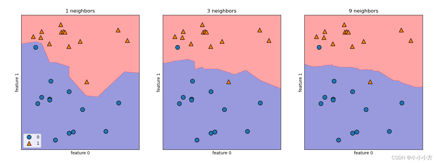
由上图可得,随着邻居个数越来越多,决策边界也越来越平滑,更平滑的边界对应更简单的模型。
探讨模型复杂程度和泛化能力之间的关系,先将数据集分成训练集和测试集,然后用不同的邻居个数对训练集和测试集的性能进行评估。
# 利用乳腺癌数据集
from sklearn.datasets import load_breast_cancer
cancer = load_breast_cancer()
x_train,x_test,y_train,y_test = train_test_split(cancer.data,cancer.target,stratify=cancer.target,random_state=66)
# 训练集精度
training_accuracy = []
# 测试集精度
test_accuracy = []
# n_neighbor取值从1到10
neighbors_settings = range(1,11)
for n_neighbors in neighbors_settings:
    # 构建模型
    clf = KNeighborsClassifier(n_neighbors = n_neighbors)
    clf.fit(x_train,y_train)
    # 记录训练集精度
    training_accuracy.append(clf.score(x_train,y_train))
    # 记录泛化的精度
    test_accuracy.append(clf.score(x_test,y_test))

plt.plot(neighbors_settings,training_accuracy,label="training accuracy")
plt.plot(neighbors_settings,test_accuracy,label="test accuracy")
plt.xlabel("accuracy")
plt.ylabel("n_neighbors")
plt.legend()
plt.show()
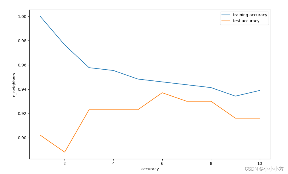
随着邻居的增多,模型变得简单,训练集精度也随着下降,测试集的精度增加,最佳性能的邻居大约在6个。
K近邻回归
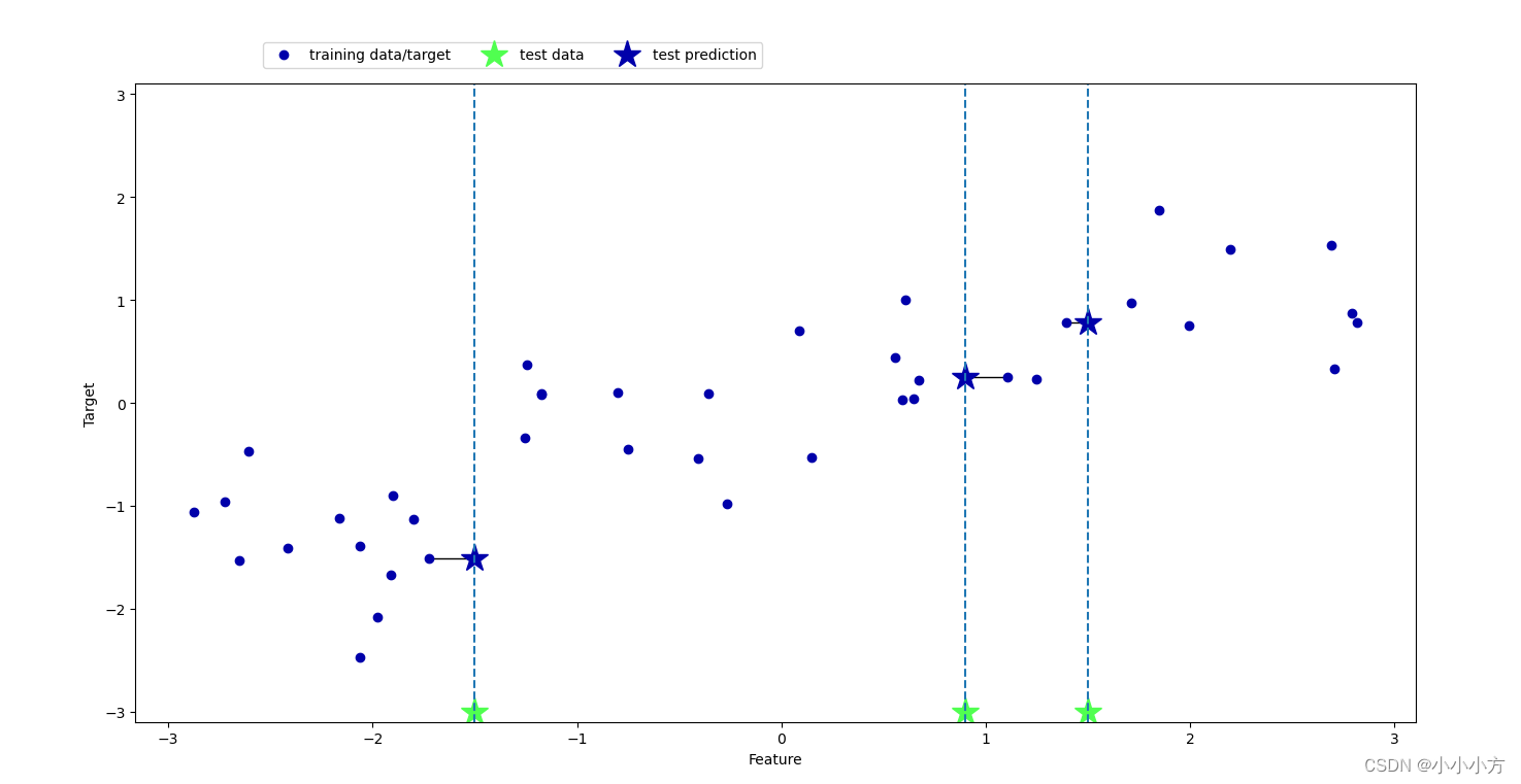
k近邻算法还可以用于回归,我们先从单一近邻开始,使用wave数据集,添加3个测试数据点。
# 单一近邻回归
mglearn.plots.plot_knn_regression(n_neighbors = 1)
plt.show()

def plot_knn_regression(n_neighbors=1):
    X, y = make_wave(n_samples=40)
    X_test = np.array([[-1.5], [0.9], [1.5]])

    dist = euclidean_distances(X, X_test)
    closest = np.argsort(dist, axis=0)
    # figure()函数自定义画布
    plt.figure(figsize=(10, 6))

    reg = KNeighborsRegressor(n_neighbors=n_neighbors).fit(X, y)
    y_pred = reg.predict(X_test)

    for x, y_, neighbors in zip(X_test, y_pred, closest.T):
        for neighbor in neighbors[:n_neighbors]:
                plt.arrow(x[0], y_, X[neighbor, 0] - x[0], y[neighbor] - y_,
                          head_width=0, fc='k', ec='k')

    train, = plt.plot(X, y, 'o', c=cm3(0))
    # test data的y值应该设置为一个数组处于最底部的数组 -3 * np.ones(len(X_test))
    test, = plt.plot(X_test, -3 * np.ones(len(X_test)), '*', c=cm3(2),
                     markersize=20)
    pred, = plt.plot(X_test, y_pred, '*', c=cm3(0), markersize=20)
    # vlines函数作用是根据x轴的位置绘制一组可设置y轴方向起始值和终止值的垂直线。
    plt.vlines(X_test, -3.1, 3.1, linestyle="--")
    plt.legend([train, test, pred],
               ["training data/target", "test data", "test prediction"],
               ncol=3, loc=(.1, 1.025))
    plt.ylim(-3.1, 3.1)
    plt.xlabel("Feature")
    plt.ylabel("Target")
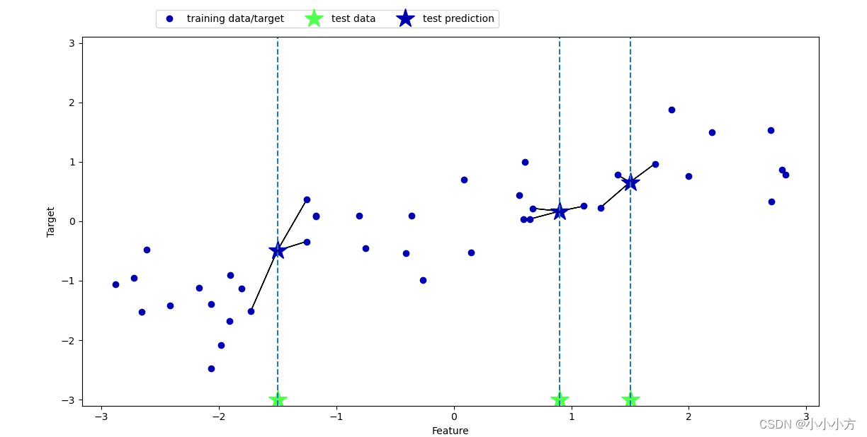
# 多个近邻回归 预测结果为这些邻居的平均值
mglearn.plots.plot_knn_regression(n_neighbors = 3)
plt.show()
用于回归的k近邻算法在scikit-learn中的实现
# 用于k近邻算法在scilit-learn的KNeighborsRegressor类中实现
from sklearn.neighbors import KNeighborsRegressor
x,y = mglearn.datasets.make_wave(n_samples = 40)
x_train,x_test,y_train,y_test = train_test_split(x,y,random_state=0)
print(x_train.shape,y_train.shape)
# 模型实例化,并将邻居的个数设置为3
reg = KNeighborsRegressor(n_neighbors = 3)
# 利用训练数据和训练目标值来拟合模型
reg.fit(x_train,y_train)
# 对测试集进行测试
print("test set prediction{}".format(reg.predict(x_test)))
# 使用score方法来评估模型,对于回归问题,这一方法返回的是R2的分数,R2分数也叫做决定稀疏,是回归模型预测的优度度量,位于0到1之间
# R2等于1对应与完美预测,等于0对应常数模型,即总是预测训练集相应y_trian的平均值
print("test set R2:{:.2f}".format(reg.score(x_test,y_test)))

运行结果:
test set prediction[-0.05396539  0.35686046  1.13671923 -1.89415682 -1.13881398 -1.63113382  0.35686046  0.91241374 -0.44680446 -1.13881398]
test set R2:0.83
对于回归问题,这一方法返回的是 R2 分数。R2 分
数也叫作决定系数,是回归模型预测的优度度量,位于 0 到 1 之间。R2 等于 1 对应完美预测,R2 等于 0 对应常数模型,即总是预测训练集响应(y_train)的平均值
分析KNeighborsRegressor
# 对于我们的一维数据集,可以查看所有特征取值对应的预测结果,创建一个由许多点组成的测试数据集
fig,axes = plt.subplots(1,3,figsize=(15,4))
# 创建1000个数据点,在-3和3之间均匀分布 转换成一列
line = np.linspace(-3,3,1000).reshape(-1,1)
for n_neighbors,ax in zip([1,3,9],axes):
    # 利用1个,3个或9个邻居分别进行预测
    reg = KNeighborsRegressor(n_neighbors=n_neighbors)
    reg.fit(x_train,y_train)
    ax.plot(line,reg.predict(line))
    ax.plot(x_train,y_train,'^',c=mglearn.cm2(0),markersize=8)
    ax.plot(x_test,y_test,'v',c=mglearn.cm2(1),markersize=8)
    ax.set_title(
        "{} neighbors\n trian score:{:.2f} test score:{:.2f}".format(
            n_neighbors,reg.score(x_train,y_train),
            reg.score(x_test,y_test)
        )
    )
    ax.set_xlabel("feature")
    ax.set_ylabel("target")
axes[0].legend(["model predictions","training data/target","test data/target"],loc="best")
plt.show()
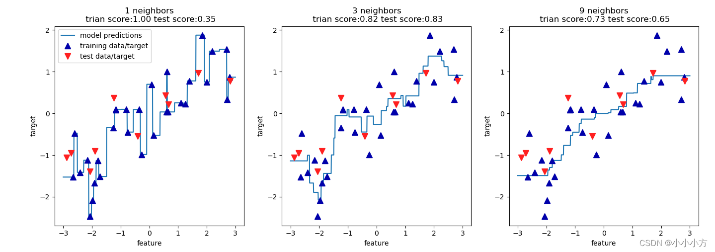
仅使用单一邻居,训练集中的每个点都对预测结果有显著影响,预测结果的图像经过所有数据点。这导致预测结果非常不稳定。考虑更多的邻居之后,预测结果变得更加平滑,但对训练数据的拟合也不好。
优点和缺点
KNeighbors 分类器有 2 个重要参数:邻居个数与数据点之间距离的度量方法。在实践中,使用较小的邻居个数(比如 3 个或 5 个)往往可以得到比较好的结果,但你应该调节这个参数。使用 k-NN 算法时,对数据进行预处理是很重要的。这一算法对于有很多特征(几百或更多)的数据集往往效果不好,对于大多数特征的大多数取值都为 0 的数据集(所谓的稀疏数据集)来说,这一算法的效果尤其不好。
3.线性模型
线性模型利用输入特征的线性函数(linear function)进行预测。
用于回归的线性模型
对于回归问题,线性模型预测的一般公式如下:
ŷ = w[0] * x[0] + w[1] * x[1] + … + w[p] * x[p] + b
这里 x[0] 到 x[p] 表示单个数据点的特征(本例中特征个数为 p+1),w 和 b 是学习模型的参数,ŷ 是模型的预测结果。对于单一特征的数据集,公式如下:
ŷ = w[0] * x[0] + b
一维 wave 数据集上学习参数 w[0] 和 b:
import numpy as np
import matplotlib.pyplot as plt
import pandas as pd
from sklearn.model_selection import train_test_split
import mglearn

# 在一维wave数据集上学习参数w[0]和b
mglearn.plots.plot_linear_regression_wave()
plt.show()

def plot_linear_regression_wave():
    X, y = make_wave(n_samples=60)
    X_train, X_test, y_train, y_test = train_test_split(X, y, random_state=42)
    line = np.linspace(-3, 3, 100).reshape(-1, 1)
    # 训练模型
    lr = LinearRegression().fit(X_train, y_train)
    # 权重或系数被保存在coef_中,偏移或截距被保留字在intercept_中
    print("w[0]: %f  b: %f" % (lr.coef_[0], lr.intercept_))
    plt.figure(figsize=(8, 8))
    plt.plot(line, lr.predict(line))
    plt.plot(X, y, 'o', c=cm2(0))
    # 获取四个坐标轴
    ax = plt.gca()
    ax.spines['left'].set_position('center')
    # 对于不需要的坐标轴进行隐藏
    ax.spines['right'].set_color('none')
    ax.spines['bottom'].set_position('center')
    ax.spines['top'].set_color('none')
    # 设置坐标轴的范围
    ax.set_ylim(-3, 3)
    #ax.set_xlabel("Feature")
    #ax.set_ylabel("Target")
    ax.legend(["model", "training data"], loc="best")
    # 设置网格
    ax.grid(True)
    # 将两个坐标轴的比例设置为一样
    ax.set_aspect('equal')

运行结果:
w[0]: 0.393906  b: -0.031804
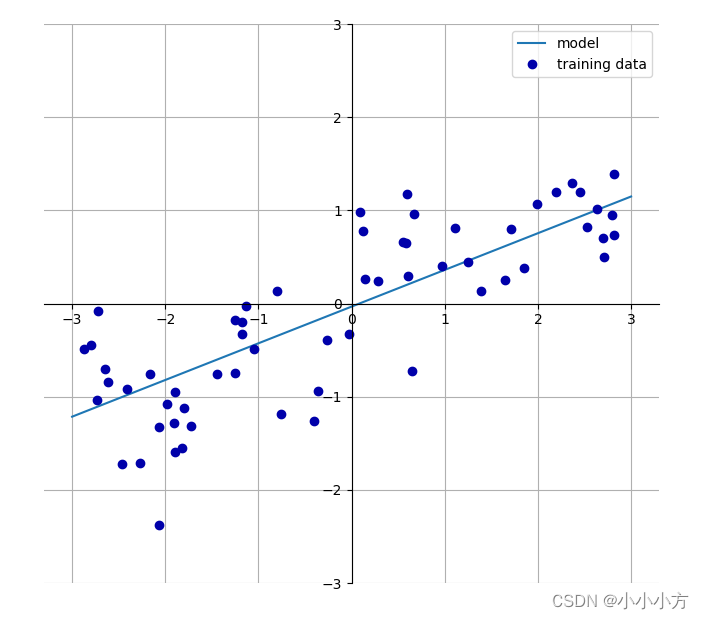
用于回归的线性模型可以表示为这样的回归模型:对单一特征的预测结果是一条直线,两个特征时是一个平面,或者在更高维度(即更多特征)时是一个超平面。
线性回归
线性回归,或者普通最小二乘法(ordinary least squares,OLS),是回归问题最简单也最经典的线性方法。线性回归寻找参数 w 和 b,使得对训练集的预测值与真实的回归目标值 y之间的均方误差最小。均方误差(mean squared error)是预测值与真实值之差的平方和除
以样本数。线性回归没有参数,这是一个优点,但也因此无法控制模型的复杂度。
# 线性回归
from sklearn.linear_model import LinearRegression
x,y = mglearn.datasets.make_wave(n_samples = 60)
x_train,x_test,y_train,y_test = train_test_split(x,y,random_state=42)
lr = LinearRegression().fit(x_train,y_train)
# 斜率参数w被保存在coef_属性中,而偏移或截距b被保存在intercept_属性中
# scikit-learn总是训练数据中得出的值保存在以下划线结尾的属性中。这是为了将其与用户设置的参数区分开
print("lr.coef_:{}".format(lr.coef_))
print("lr.intercept_:{}".format(lr.intercept_))
# intercept_属性是一个浮点数,coef_属性是一个numpy数组,每个元素对应一个输入特征
# 但是wave数据集中只有一个输入特征,所有lr.coef_中只有一个元素
print("trianing set score:{:.2f}".format(lr.score(x_train,y_train)))
print("test set score:{:.2f}".format(lr.score(x_test,y_test)))
运行结果:
lr.coef_:[0.39390555]
lr.intercept_:-0.031804343026759746
trianing set score:0.67
test set score:0.66
这个结果不是很好,但我们可以看到,训练集和测试集上的分数非常接近。这说明可能存在欠拟合,而不是过拟合。对于这个一维数据集来说,过拟合的风险很小,因为模型非常简单(或受限)。然而,对于更高维的数据集(即有大量特征的数据集),线性模型将变得更加强大,过拟合的可能性也会变大。
LinearRegression 在更复杂的数据集上的表现
# 使用线性回归在更复杂的数据集上的表现 波士顿房价数据集
x,y = mglearn.datasets.load_extended_boston()
x_train,x_test,y_train,y_test = train_test_split(x,y,random_state=0)
lr = LinearRegression().fit(x_train,y_train)
print("trianing set score:{:.2f}".format(lr.score(x_train,y_train)))
print("test set score:{:.2f}".format(lr.score(x_test,y_test)))
运行结果:
trianing set score:0.95
test set score:0.61
训练集和测试集之间的性能差异是过拟合的明显标志。
岭回归
岭回归也是一种用于回归的线性模型,因此它的预测公式与普通最小二乘法相同。但在岭回归中,对系数(w)的选择不仅要在训练数据上得到好的预测结果,而且还要拟合附加约束。我们希望系数尽量小。换句话说,w 的所有元素都应接近于 0。直观上来看,这意味着每个特征对输出的影响应尽可能小(即斜率很小),同时仍给出很好的预测结果。这种约束是所谓正则化的一个例子。正则化是指对模型做显式约束,以监督学习避免过拟合。岭回归用到的这种被称为 L2 正则化。
模型权重数量不宜太多,权重的取值范围应尽量一致,权重越小拟合能力越差,有利于防止过拟合。
# 岭回归在 linear_model.Ridge 中实现
from sklearn.linear_model import Ridge
ridge = Ridge().fit(x_train,y_train)
print("  set score:{:.2f}".format(ridge.score(x_train,y_train)))
print("test set score:{:.2f}".format(ridge.score(x_test,y_test)))
运行结果:
 set score:0.89
test set score:0.75
Ridge 在训练集上的分数要低于 LinearRegression,但在测试集上的分数更高。简单性和训练集性能二者对于模型的重要程度可以由用户通过设置 alpha 参数来指定。在前面的例子中,我们用的是默认参数 alpha=1.0。但没有理由认为这会给出最佳权衡。alpha 的最佳设定
值取决于用到的具体数据集。
ridge10 = Ridge(alpha=10).fit(x_train,y_train)
print("trianing set score:{:.2f}".format(ridge10.score(x_train,y_train)))
print("test set score:{:.2f}".format(ridge10.score(x_test,y_test)))
ridge01 = Ridge(alpha=0.1).fit(x_train,y_train)
print("trianing set score:{:.2f}".format(ridge01.score(x_train,y_train)))
print("test set score:{:.2f}".format(ridge01.score(x_test,y_test)))

运行结果:
trianing set score:0.79
test set score:0.64
trianing set score:0.93
test set score:0.77
增大 alpha 会使得系数更加趋向于 0,从而降低训练集性能,但可能会提高泛化性能。减小 alpha 可以让系数受到的限制更小。
查看 alpha 取不同值时模型的 coef_ 属性:
plt.plot(ridge.coef_,'s',label= "Ridge alpha = 1")
plt.plot(ridge10.coef_,'^',label= "Ridge alpha = 10")
plt.plot(ridge01.coef_,'v',label= "Ridge alpha = 01")
plt.plot(lr.coef_,'o',label = "linearRegession")
plt.xlabel("coefficient index")
plt.ylabel("coefficient magnitude")
# 根据y轴的位置绘制一组可设置x轴方向起始值和终止值的水平线
plt.hlines(0,0,len(lr.coef_))
plt.ylim(-25,25)
# 在plot()之后显示label的内容
plt.legend()
plt.show()
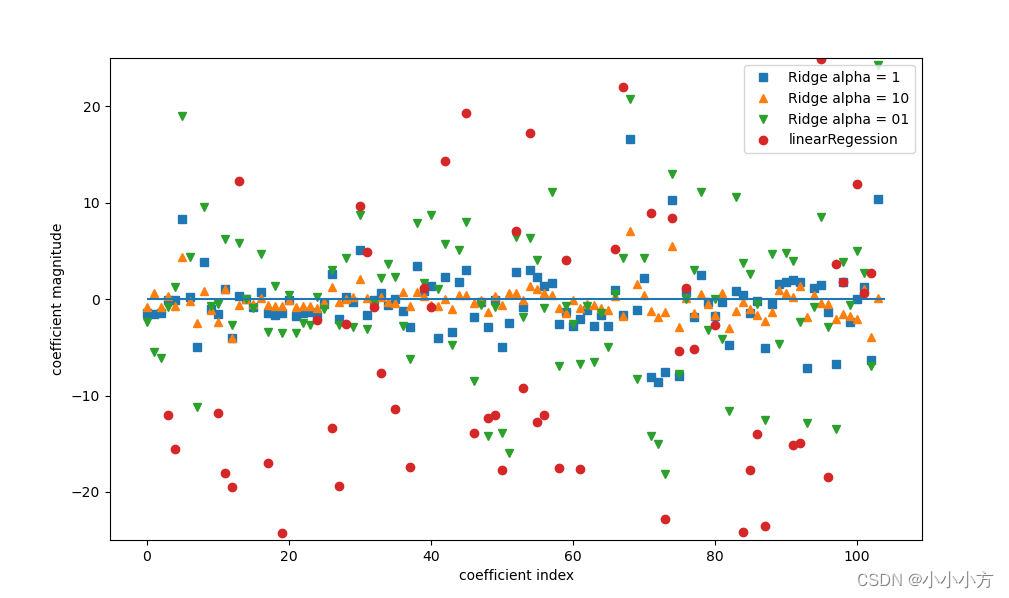
alpha不同的线性模型之间的系数值波动范围。
是固定 alpha 值,但改变训练数据量,来理解正则化的影响:
对波士顿房价数据集做二次抽样,并在数据量逐渐增加的子数据集上分别对 LinearRegression 和 Ridge(alpha=1) 两个模型进行评估(将模型性能作为数据集大小的函数进行绘图,这样的图像叫作学习曲线):
mglearn.plots.plot_ridge_n_samples()
plt.show()
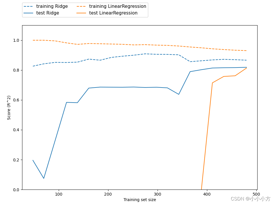
随着模型可用的数据越来越多,两个模型的性能都在提升,最终
线性回归的性能追上了岭回归。这里要记住的是,如果有足够多的训练数据,正则化变得不那么重要,并且岭回归和线性回归将具有相同的性能。与此同时,线性回归的训练性能在下降。如果添加更多数据,模型将更加难以过拟合或记住所有的数据。
lasso
与岭回归相同,使用 lasso 也是约束系数使其接近于 0,但用到的方法不同,叫作 L1 正则化。 L1 正则化的结果是,使用 lasso 时某些系数刚好为 0。这说明某些特征被模型完全忽略。这可以看作是一种自动化的特征选择。
# lasso
from sklearn.linear_model import Lasso
lasso = Lasso().fit(x_train,y_train)
print("trianing set score:{:.2f}".format(lasso.score(x_train,y_train)))
print("test set score:{:.2f}".format(lasso.score(x_test,y_test)))
print("Number of features used:{}".format(np.sum(lasso.coef_!= 0)))
运行结果:
trianing set score:0.29
test set score:0.21
Number of features used:4
Lasso 也有一个正则化参数 alpha,可以控制系数趋向于 0 的强度。在上一个例子中,我们用的是默认值 alpha=1.0。为了降低欠拟
合,我们尝试减小 alpha。这么做的同时,我们还需要增加 max_iter 的值(运行迭代的最大次数):
lasso001 = Lasso(alpha=0.01,max_iter=100000).fit(x_train,y_train)
print("trianing set score:{:.2f}".format(lasso001.score(x_train,y_train)))
print("test set score:{:.2f}".format(lasso001.score(x_test,y_test)))
print("Number of features used:{}".format(np.sum(lasso001.coef_!= 0)))
运行结果:
trianing set score:0.90
test set score:0.77
Number of features used:33
但如果把 alpha 设得太小,那么就会消除正则化的效果,并出现过拟合
lasso00001 = Lasso(alpha=0.0001,max_iter=100000).fit(x_train,y_train)
print("trianing set score:{:.2f}".format(lasso00001.score(x_train,y_train)))
print("test set score:{:.2f}".format(lasso00001.score(x_test,y_test)))
print("Number of features used:{}".format(np.sum(lasso00001.coef_!= 0)))
运行结果:
trianing set score:0.95
test set score:0.64
Number of features used:96
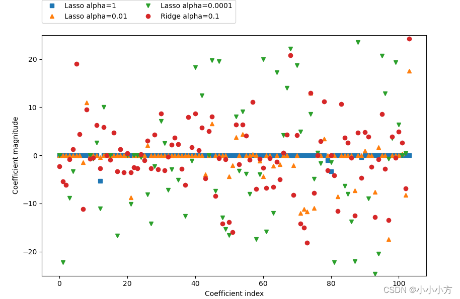
对不同模型的系数进行作图
plt.plot(lasso.coef_, 's', label="Lasso alpha=1")
plt.plot(lasso001.coef_, '^', label="Lasso alpha=0.01")
plt.plot(lasso00001.coef_, 'v', label="Lasso alpha=0.0001")
plt.plot(ridge01.coef_, 'o', label="Ridge alpha=0.1")
plt.legend(ncol=2, loc=(0, 1.05))
plt.ylim(-25, 25)
plt.xlabel("Coefficient index")
plt.ylabel("Coefficient magnitude")
plt.show()
用于分类的线性模型
线性模型也广泛应用于分类问题。我们首先来看二分类。这时可以利用下面的公式进行预测:
ŷ = w[0] * x[0] + w[1] * x[1] + …+ w[p] * x[p] + b > 0
这个公式看起来与线性回归的公式非常相似,但我们没有返回特征的加权求和,而是为预测设置了阈值(0)。如果函数值小于 0,我们就预测类别 -1;如果函数值大于 0,我们就预测类别 +1。对于所有用于分类的线性模型,这个预测规则都是通用的。同样,有很多种
不同的方法来找出系数(w)和截距(b)。对于用于回归的线性模型,输出 ŷ 是特征的线性函数,是直线、平面或超平面(对于更高
维的数据集)。对于用于分类的线性模型,决策边界是输入的线性函数。换句话说,(二元)线性分类器是利用直线、平面或超平面来分开两个类别的分类器。
最常见的两种线性分类算法是 Logistic 回归(logistic regression)和线性支持向量机(linear support vector machine,线性 SVM)
我们可以将 LogisticRegression 和 LinearSVC 模型应用到 forge 数据集上,并将线性模型找到的决策边界可视化
import numpy as np
import matplotlib.pyplot as plt
import pandas as pd
from sklearn.model_selection import train_test_split
import mglearn
from sklearn.linear_model import LogisticRegression
from sklearn.svm import LinearSVC
x,y = mglearn.datasets.make_forge()
fig,axes = plt.subplots(1,2,figsize =(10,3))
for model,ax in zip([LinearSVC(),LogisticRegression()],axes):
    clf = model.fit(x,y)  mglearn.plots.plot_2d_separator(clf,x,fill=False,eps=0.5,ax=ax,alpha=0.7)
    mglearn.discrete_scatter(x[:,0],x[:,1],y,ax=ax)
    ax.set_title("{}".format(clf.__class__.__name__))
    ax.set_xlabel("feature 0")
    ax.set_ylabel("feature 1")
axes[0].legend()
plt.show()
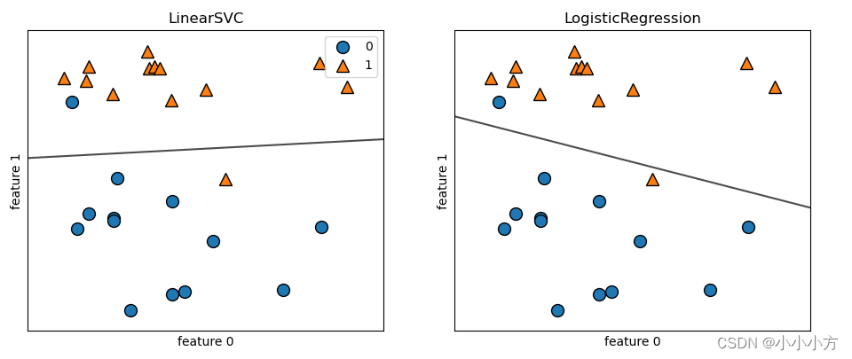
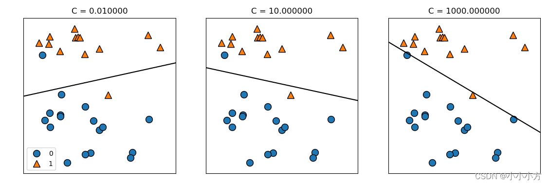
两个模型得到了相似的决策边界,都存在两个点的分类是错误的,都默认使用了L2正则化。对于LogisticRegression和LinearSVC来说,决定正则化强度的权衡参数是C,C值越大对应的正则化越若弱。
较小的C值可以让算法尽量适应“大多数”数据点,较大的C值更强调每个数据点都分类正确的正确性。
用于分类的线性模型在低维空间中看起来非常受限,决策边界只能是直线或平面。在高维空间中,用于分类的线性模型变得非常强大,当考虑更多特征时,避免过拟合变得重要。
我们在乳腺癌数据集上详细分析 LogisticRegression:
from sklearn.datasets import load_breast_cancer
cancer = load_breast_cancer()
x_train,x_test,y_train,y_test = train_test_split(cancer.data,cancer.target,stratify=cancer.target,random_state=42)
logreg = LogisticRegression().fit(x_train,y_train)
print("training set score{:.3f}".format(logreg.score(x_train,y_train)))
print("test set score{:03f}".format(logreg.score(x_test,y_test)))

运行结果:
training set score0.946
test set score0.958042
C=1 的默认值给出了相当好的性能,在训练集和测试集上都达到 95% 的精度。但由于训练集和测试集的性能非常接近,所以模型很可能是欠拟合的。
logreg100 = LogisticRegression(C=100).fit(x_train,y_train)
print("training set score{:.3f}".format(logreg100.score(x_train,y_train)))
print("test set score{:03f}".format(logreg100.score(x_test,y_test)))

运行结果:
Training set score: 0.972
Test set score: 0.965
logreg001 = LogisticRegression(C=0.01).fit(X_train, y_train)
print("Training set score: {:.3f}".format(logreg001.score(X_train, y_train)))
print("Test set score: {:.3f}".format(logreg001.score(X_test, y_test)))

运行结果:
Training set score: 0.934
Test set score: 0.930
最后,正则化参数 C 取三个不同的值时模型学到的系数
plt.plot(logreg.coef_.T,'o',label="C=1")
plt.plot(logreg100.coef_.T,'^',label="C=100")
plt.plot(logreg001.coef_.T,'v',label="C=001")
# 设置x轴的刻度和标签
plt.xticks(range(cancer.data.shape[1]), cancer.feature_names, rotation=90)
plt.hlines(0,0,cancer.data.shape[1])
plt.ylim(-5,5)
plt.xlabel("coefficient index")
plt.ylabel("coefficient magnitude")
plt.legend()
plt.show()
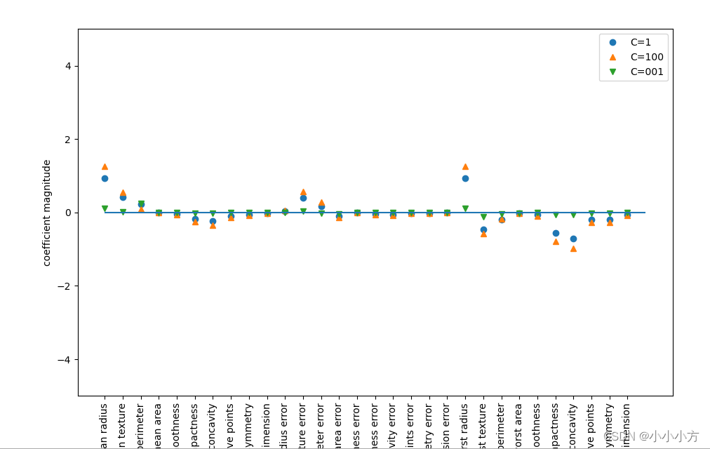
使用L1正则化的模型,约束模型只使用少数特征。
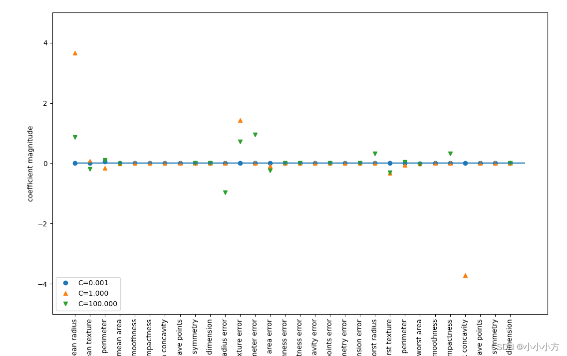
for C,marker in zip([0.001,1,100],['o','^','v']):
    lr_l1 = LogisticRegression(C=C,penalty="l1",solver='liblinear').fit(x_train,y_train)
    print("training accuracy of l1 logreg with c={:.3f}:{:.2f}".format(C,lr_l1.score(x_train,y_train)))
    print("test accuracy of l1 logreg with c={:.3f}:{:.2f}".format(C, lr_l1.score(x_test, y_test)))
    plt.plot(lr_l1.coef_.T,marker,label = "C={:.3f}".format(C))
    plt.xticks(range(cancer.data.shape[1]),cancer.feature_names,rotation=90)
    plt.hlines(0,0,cancer.data.shape[1])
    plt.xlabel("coefficient index")
    plt.ylabel("coefficient magnitude")
    plt.ylim(-5,5)
    plt.legend(loc=3)
plt.show()

运行结果:
training accuracy of l1 logreg with c=0.001:0.91
test accuracy of l1 logreg with c=0.001:0.92
training accuracy of l1 logreg with c=1.000:0.96
test accuracy of l1 logreg with c=1.000:0.96
training accuracy of l1 logreg with c=100.000:0.99
test accuracy of l1 logreg with c=100.000:0.98
用于二分类的线性模型与用于回归的线性模型有许多相似之处。与用于回归的线性模型一样,模型的主要差别在于 penalty 参数(使用L1正则化还是L2),这个参数会影响正则化,也会影响模型是使用所有可用特征还是只选择特征的一个子集。
用于多分类的线性模型
将二分类算法推广到多分类算法的一种常见方法是“一对其余”方法。在“一对其余”方法中,对每个类别都学习一个二分类模型,将这个类别与所有其他类别尽量分开,这样就生成了与类别个数一样多的二分类模型。在测试点上运行所有二类分类器来进行预测。在对应类别上分数最高的分类器“胜出”,将这个类别标签返回作为预测结果。
每个类别都对应一个二类分类器,这样每个类别也都有一个系(w)向量和一个截距(b)。下面给出的是分类置信方程,其结果中最大值对应的类别即为预测的类别标签:
w[0] * x[0] + w[1] * x[1] + … + w[p] * x[p] + b
多分类 Logistic 回归背后的数学与“一对其余”方法稍有不同,但它也是对每个类别都有一个系数向量和一个截距,也使用了相同的预测方法。
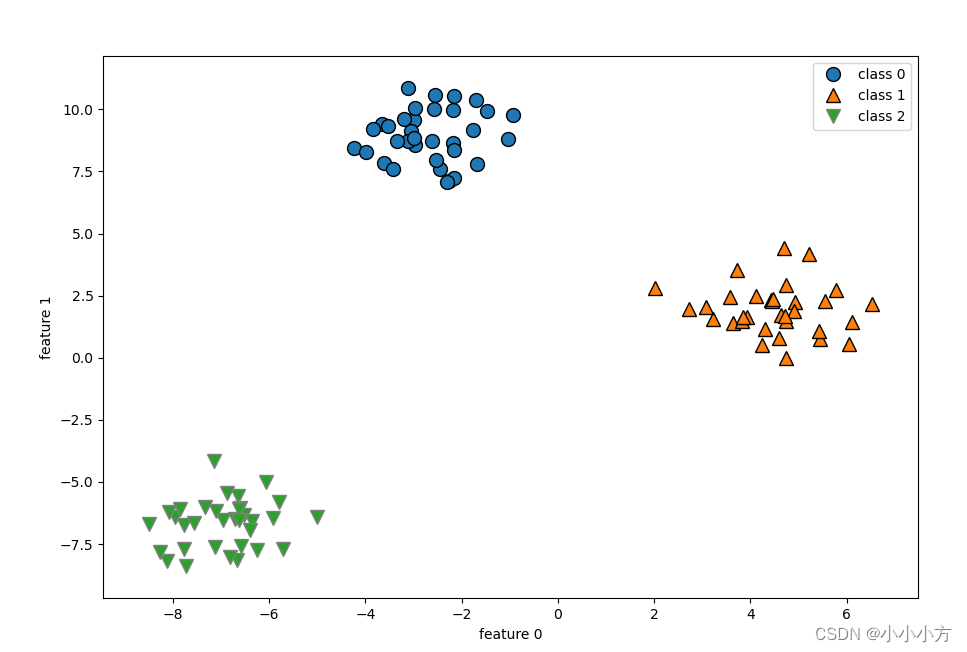
# 将一对其余的方法应用在一个简单的三分类数据集上
from sklearn.datasets import make_blobs
x,y = make_blobs(random_state=42)
mglearn.discrete_scatter(x[:,0],x[:,1],y)
plt.xlabel("feature 0")
plt.ylabel("feature 1")
plt.legend(["class 0","class 1","class 2"])
plt.show()
在这个数据集上训练一个 LinearSVC 分类器:
linear_svm = LinearSVC().fit(x,y)
print("cofficient shape:",linear_svm.coef_.shape)
print("intercept shape:",linear_svm.intercept_.shape)
运行结果:
cofficient shape: (3, 2)
intercept shape: (3,)
coef_ 的形状是 (3, 2),说明 coef_ 每行包含三个类别之一的系数向量,每列包含某个特征(这个数据集有 2 个特征)对应的系数值。现在 intercept_ 是一维数组,保存每个类别的截距。
我们将这 3 个二类分类器给出的直线可视化
mglearn.discrete_scatter(x[:,0],x[:,1],y)
line = np.linspace(-15,15)
for coef,intercept,color in zip(linear_svm.coef_,linear_svm.intercept_,['b','r','g']):
    plt.plot(line,-(line*coef[0]+intercept)/coef[1],c=color)
plt.ylim(-10,15)
plt.ylim(-10,8)
plt.xlabel("feature 0")
plt.ylabel("feature 1")
plt.legend(['class 0','class 1','class 2','line class 1','line class 1','line class 2'],loc=(1.01,0.3))
plt.show()
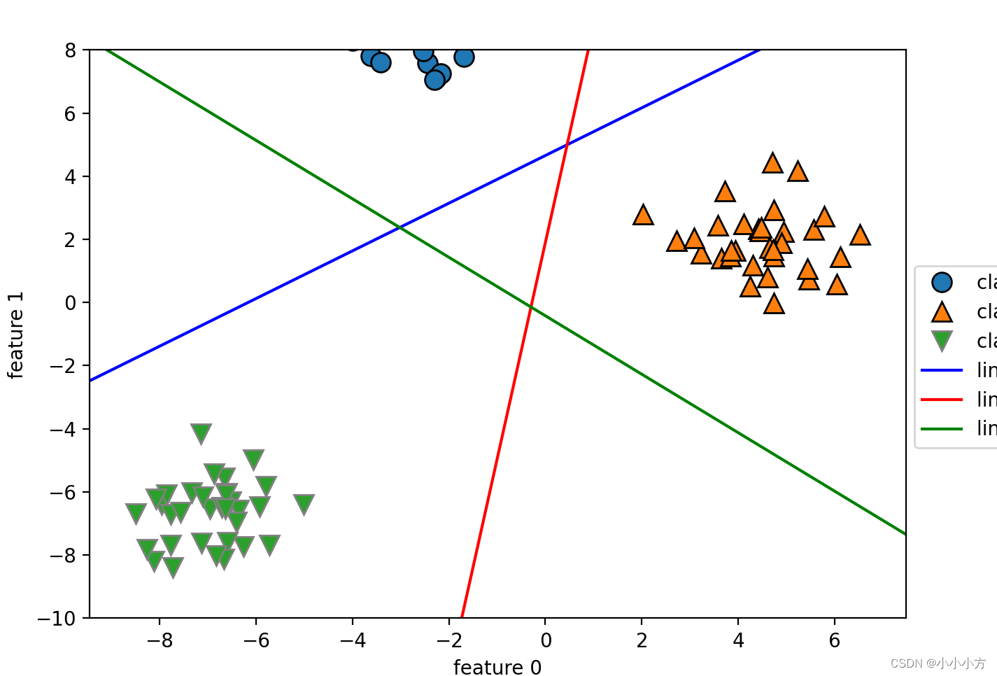
但图像中间的三角形区域属于最接近的那条线对应的类别
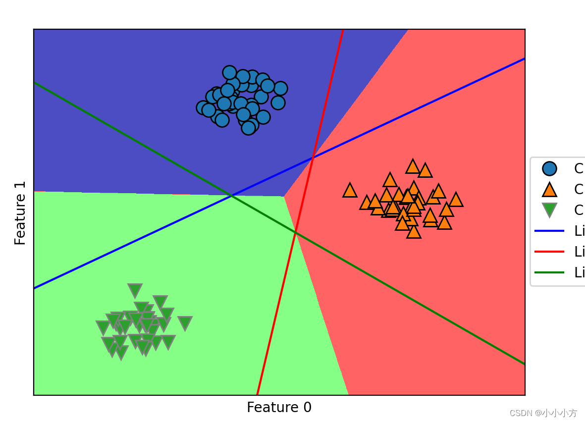
# 给出二维空间种所有区域的预测结果
mglearn.plots.plot_2d_classification(linear_svm, x, fill=True, alpha=.7)
mglearn.discrete_scatter(x[:, 0], x[:, 1], y)
line = np.linspace(-15, 15)
for coef, intercept, color in zip(linear_svm.coef_, linear_svm.intercept_,['b', 'r', 'g']):
    plt.plot(line, -(line * coef[0] + intercept) / coef[1], c=color)
plt.legend(['Class 0', 'Class 1', 'Class 2', 'Line class 0', 'Line class 1','Line class 2'], loc=(1.01, 0.3))
plt.xlabel("Feature 0")
plt.ylabel("Feature 1")
plt.show()
优点缺点
线性模型的主要参数是正则化参数,alpha 值较大或 C 值较小,说明模型比较简单。特别是对于回归模型而言,调节这些参数非常重要。通常在对数尺度上对 C 和 alpha 进行搜索。线性模型的训练速度非常快,预测速度也很快。这种模型可以推广到非常大的数据集,对
稀疏数据也很有效。如果你的数据包含数十万甚至上百万个样本,你可能需要研究如何使用 LogisticRegression 和 Ridge 模型的 solver=‘sag’ 选项,在处理大型数据时,这一选项比默认值要更快。
如果特征数量大于样本数量,线性模型的表现通常都很好。它也常用于非常大的数据集,只是因为训练其他模型并不可行。但在更低维的空间中,其他模型的泛化性能可能更好。


 被折叠的 条评论
为什么被折叠?
被折叠的 条评论
为什么被折叠?
 到【灌水乐园】发言


