Matplotlib Introductory Basic Usage-优快云博客

本文链接：https://blog.youkuaiyun.com/weixin_55688821/article/details/130768931

Introductory

总览

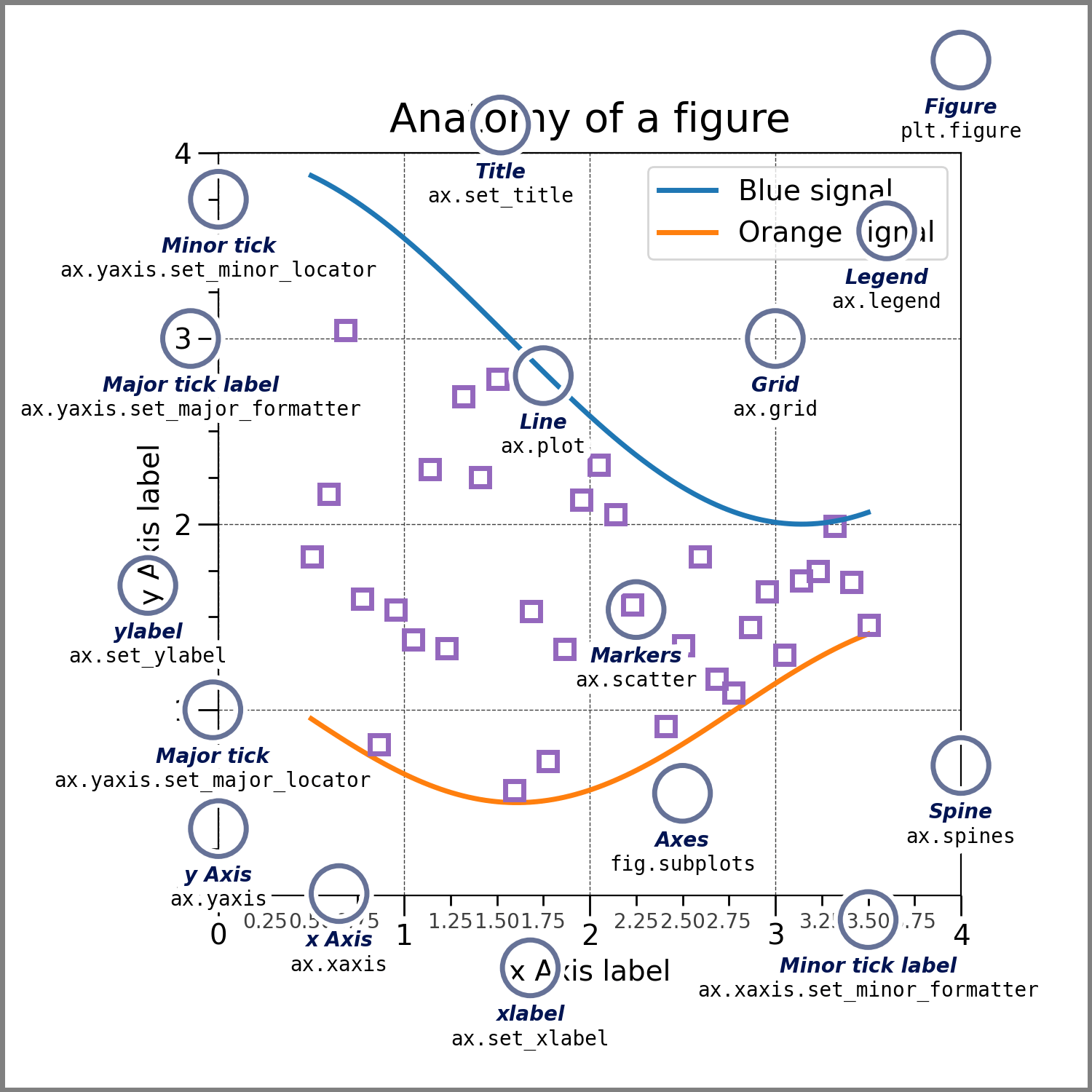
介绍了Matplotlib的基本用法, Figure, Axes, Axis, Artist等基本的类. 函数包括

ax1.twinx() 生成一个Axes 共享ax1的x轴

ax3.secondary_xaxis(position, functions) 给 ax3 添加一个 x 轴

返回值ax : axes._secondary_axes.SecondaryAxis

pcolormesh(), contourf(), imshow(), scatter()

fig.colorbar(mappable, cax=None, ax=None, use_gridspec=True, **kw) 颜色条

subplot_mosiac() 设计更复杂的布局

Basic Usage

Axis

设置比例和范围, 生成刻度和刻度标签.
The location of the ticks is determined by a Locator object and the ticklabel strings are formatted by a Formatter.The combination of the correct Locator and Formatter gives very fine control over the tick locations and labels.

Artist

基本上所有可见的东西都是Aritist对象(包括Figure, Axes, Axis对象等)

两种风格

面对对象风格(建议)
ax.
pyplot风格
plt.

Styling Artists

fig, ax = plt.subplots(figsize=(5, 2.7))
x = np.arange(len(data1))
ax.plot(x, np.cumsum(data1), color='blue', linewidth=3, linestyle='--')
l, = ax.plot(x, np.cumsum(data2), color='orange', linewidth=2) # <matplotlib.lines.Line2D at 0x2c6d0d5aac0>
l.set_linestyle(':');
# l = ax.plot(x, np.cumsum(data2), color='orange', linewidth=2) # [<matplotlib.lines.Line2D at 0x2c6d0d5aac0>]

l 是一个Line2D 类型的对象利用其设置线的参数. 由于plot返回列表所以就加个逗号, 等同于l[0]

Labelling plots

set_xlabel, set_ylabel, and set_title are used to add text in the indicated locations (see Text in Matplotlib Plots for more discussion). Text can also be directly added to plots using text:
这些text函数都会返回Text类的实例.

Axis scales and ticks

Tick locators and formatters

不同的scale(比例尺)有不同的locators和formatters ,例如log-scale 用的是LogLocator 和 LogFormatter

Plotting dates and strings

fig, ax = plt.subplots(figsize=(5, 2.7), layout='constrained')
dates = np.arange(np.datetime64('2021-11-15'), np.datetime64('2021-12-25'),
                  np.timedelta64(1, 'h'))
data = np.cumsum(np.random.randn(len(dates)))
ax.plot(dates, data)
cdf = mpl.dates.ConciseDateFormatter(ax.xaxis.get_major_locator())
ax.xaxis.set_major_formatter(cdf)

代码没看懂, 以后再说.

Additional Axis objects

twinx() 生成一个坐标系, 但是x轴不可见, y轴被放在了右边.

t = np.arange(0.0, 5.0, 0.01)
s = np.cos(2 * np.pi * t)
fig, (ax1, ax3) = plt.subplots(1, 2, figsize=(7, 2.7), layout='constrained')
l1, = ax1.plot(t, s)
ax2 = ax1.twinx()
l2, = ax2.plot(t, range(len(t)), 'C1')
ax2.legend([l1, l2], ['Sine (left)', 'Straight (right)'])

ax3.plot(t, s)
ax3.set_xlabel('Angle [rad]')
ax4 = ax3.secondary_xaxis('top', functions=(np.rad2deg, np.deg2rad))
ax4.set_xlabel('Angle [°]')

secondary_xaxis(position, functions)
这个元组包含了弧度和角度的转化.

position表示第二条轴的位置可以为 ‘top’ ,‘bottom’, ‘left’, ‘right’
functions必须是一个二元的元组, 两个函数必须是可以互相转换的.

location : {'top', 'bottom', 'left', 'right'} or float
    The position to put the secondary axis.  Strings can be 'top' or
    'bottom' for orientation='x' and 'right' or 'left' for
    orientation='y'. A float indicates the relative position on the
    parent axes to put the new axes, 0.0 being the bottom (or left)
    and 1.0 being the top (or right).

functions : 2-tuple of func, or Transform with an inverse

    If a 2-tuple of functions, the user specifies the transform
    function and its inverse.  i.e.
    ``functions=(lambda x: 2 / x, lambda x: 2 / x)`` would be an
    reciprocal transform with a factor of 2. Both functions must accept
    numpy arrays as input.

    The user can also directly supply a subclass of
    `.transforms.Transform` so long as it has an inverse.

这个例子,functions=(lambda x: 2 / x, lambda x: 2 / x) 可能有点令人困惑, 一个数设为 a 通过第一个函数变为 2 / a 通过第二个函数又变为a.
${2\over{2\over{a}}}= {2}\times {{a}\over{2}} = a$
这两个函数实现了 a 和 2 / a 的转化.

Color mapped data

让一个图的第三维由色图里的颜色展示出来.

X, Y = np.meshgrid(np.linspace(-3, 3, 128), np.linspace(-3, 3, 128))
Z = (1 - X/2 + X**5 + Y**3) * np.exp(-X**2 - Y**2)

fig, axs = plt.subplots(2, 2, layout='constrained')
pc = axs[0, 0].pcolormesh(X, Y, Z, vmin=-1, vmax=1, cmap='RdBu_r')
fig.colorbar(pc, ax=axs[0, 0])
axs[0, 0].set_title('pcolormesh()')

co = axs[0, 1].contourf(X, Y, Z, levels=np.linspace(-1.25, 1.25, 11))
fig.colorbar(co, ax=axs[0, 1])
axs[0, 1].set_title('contourf()')

pc = axs[1, 0].imshow(Z**2 * 100, cmap='plasma',
                          norm=mpl.colors.LogNorm(vmin=0.01, vmax=100))
fig.colorbar(pc, ax=axs[1, 0], extend='both')
axs[1, 0].set_title('imshow() with LogNorm()')

pc = axs[1, 1].scatter(data1, data2, c=data3, cmap='RdBu_r')
fig.colorbar(pc, ax=axs[1, 1], extend='both')
axs[1, 1].set_title('scatter()')

pcolormesh 绘制颜色分布
X 和 Y 是数组，分别表示二维数据中的横轴和纵轴值；
Z 是一个二维数组，包含了在 (X, Y) 坐标系下的数据值；
vmin 和 vmax 是可选参数，用于设置颜色分布的最小值和最大值，默认值为 None，代表使用 Z 数组中的最小值和最大值作为范围；

fig.colorbar(mappable, cax=None, ax=None, use_gridspec=True, **kw)

参数mappable理解起来就是我们需要提供一个可以映射颜色的对象，这个对象就是我们作的图
参数ax用来指示colorbar()获取到的渐变色条在哪里显示, 可以给ax参数设置成多个Axes对象，这样一个色条就可以包括多个子图.
contourf
X 和 Y 是数组，分别表示二维数据中的横轴和纵轴值；
Z 是一个二维数组，包含了在 (X, Y) 坐标系下的数据值；
levels 是可选参数，用于设置绘制等值线的值，默认使用自动计算的值；
contourf() 函数绘制等值线，并填充不同等级的区域。
imshow
Z 是一个二维数组，包含了要在图像中显示的数据；
cmap 是可选参数，用于设置颜色映射表的名称，例如使用内置的 “plasma” 颜色映射表；
norm 是可选参数，用于设置归一化范围，例如 LogNorm 通过对数变换将数据范围转换到一个对数缩放的范围内。

imshow() 函数通常用于在坐标系中绘制灰度图或颜色分布，可以根据需求进行多种参数设置。在上述代码中，为了能更好地显示数据的变化范围，使用了 Z**2 * 100 对数据进行了平方和缩放的操作。同时，为了将数据的特点突出显示，将归一化参数设置为了 LogNorm，这样可以将颜色的变化范围控制在了一个较小的范围内，方便观察数据的变化情况。

scatter
cmap 参数只有当c是一个浮点数组时才可用.

Normalizations

归一化, 标准化

Working with multiple Figures and Axes

You can open multiple Figures with multiple calls to fig = plt.figure() or fig2, ax = plt.subplots(). By keeping the object references you can add Artists to either Figure.

Multiple Axes can be added a number of ways, but the most basic is plt.subplots() as used above. One can achieve more complex layouts, with Axes objects spanning columns or rows, using subplot_mosaic.

subplot_mosaic 设计更复杂的布局

plt.subplot_mosaic([['A panel', 'A panel', 'edge'],
					['C panel', '.',       'edge']])
'''
- 'A panel' which is 1 row high and spans the first two columns
    - 'edge' which is 2 rows high and is on the right edge
    - 'C panel' which in 1 row and 1 column wide in the bottom left
    - a blank space 1 row and 1 column wide in the bottom center
'''
'''
实际上Apnel在第一行 两列宽, edge在第三列两行宽.
Cpanel在第二行一列宽, 一个空格在第二行第二列 (. 表示空)

也可以用字符串来表示(注意只能用一个字母)

plt.subplot_mosaic('''
      AAE
      C.E
      ''')
'''
If input is a str, then it must be of the form ::

      '''
      AAE
      C.E
      '''

    where each character is a column and each line is a row.
    This only allows only single character Axes labels and does
    not allow nesting but is very terse.
'''