


注:仅仅是学习记录笔记,搬运了学习课程的ppt内容,本意不是抄袭!望大家不要误解!纯属学习记录笔记!!!!!!
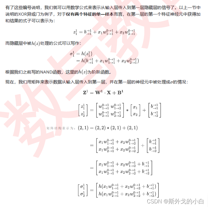
一、异或门问题
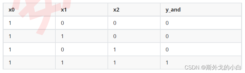
与门:一组只有两个特征(x1,x2)的分类数据,当两个特征下的取值都为1时,分类标签为1,其他时候分类标签为0。
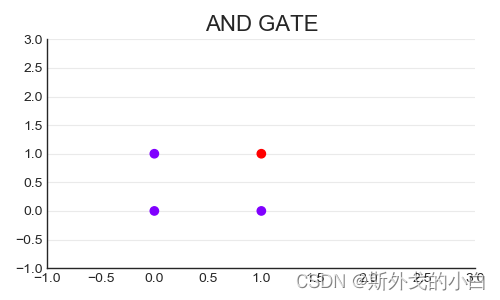
考虑到与门的数据只有两维,我们可以将数据可视化,其中,特征x1是横坐标,x2是纵坐标,紫色点代表了类别0,红色点代表类别1
import torch
import numpy as np
from matplotlib import pyplot as plt
import seaborn as sns

X = torch.tensor([[1, 0, 0], [1, 1, 0], [1, 0, 1], [1, 1, 1]],

def LogisticR(X,w):
    zhat = torch.mv(X,w) #首先执行线性回归的过程,依然是mv函数,让矩阵与向量相乘得到z
    sigma = torch.sigmoid(zhat) #执行sigmoid函数,你可以调用torch中的sigmoid函数,也可以自己用torch.exp来写
    andhat = torch.tensor([int(x) for x in sigma >= 0.5], dtype=torch.float32)
#设置阈值为0.5, 使用列表推导式将值转化为0和1
    return sigma, andhat

sigma, andhat = LogisticR(X,w)

plt.style.use('seaborn-whitegrid') #设置图像的风格
sns.set_style("white")
plt.figure(figsize=(5, 3)) #设置画布大小
plt.title("AND GATE",fontsize=16) #设置图像标题
plt.scatter(X[:, 1], X[:, 2], c=andgate, cmap="rainbow") #绘制散点图
plt.xlim(-1, 3) #设置横纵坐标尺寸
plt.ylim(-1, 3)
plt.grid(alpha=.4, axis="y") #显示背景中的网格
plt.gca().spines["top"].set_alpha(.0) #让上方和右侧的坐标轴被隐藏
plt.gca().spines["right"].set_alpha(.0)
plt.show()
import torch

X = torch.tensor([[1, 0, 0], [1, 1, 0], [1, 0, 1], [1, 1, 1]], dtype=torch.float32)
andgate = torch.tensor([0, 0, 0, 1], dtype=torch.float32)

def AND(X):
    w = torch.tensor([-0.2, 0.15, 0.15], dtype=torch.float32)
    zhat = torch.mv(X, w)
    andgate = torch.tensor([torch.ceil(x) for x in zhat], dtype=torch.float32)
    return andgate

andgate = AND(X)

print(andgate)
#tensor([0., 0., 0., 1.])

import torch
import numpy as np
from matplotlib import pyplot as plt
import seaborn as sns

X = torch.tensor([[1, 0, 0], [1, 1, 0], [1, 0, 1], [1, 1, 1]], dtype=torch.float32)
andgate = torch.tensor([0, 0, 0, 1], dtype=torch.float32)

#定义w


def AND(X):
    w = torch.tensor([-0.2, 0.15, 0.15], dtype=torch.float32)
    zhat = torch.mv(X, w)
    andgate = torch.tensor([torch.ceil(x) for x in zhat], dtype=torch.float32)
    return andgate

andhat = AND(X)

print(andgate)
#tensor([0., 0., 0., 1.])


plt.style.use('seaborn-whitegrid') #设置图像的风格
sns.set_style("white")
plt.figure(figsize=(5, 3)) #设置画布大小
plt.title("AND GATE",fontsize=16) #设置图像标题
plt.scatter(X[:, 1], X[:, 2], c=andgate, cmap="rainbow") #绘制散点图
plt.xlim(-1, 3) #设置横纵坐标尺寸
plt.ylim(-1, 3)
plt.grid(alpha=.4, axis="y") #显示背景中的网格
plt.gca().spines["top"].set_alpha(.0) #让上方和右侧的坐标轴被隐藏
plt.gca().spines["right"].set_alpha(.0)
x = np.arange(-1.3, 3.0)
plt.plot(x, (0.23-0.15*x)/0.15, color='k', linestyle='--')
plt.show()
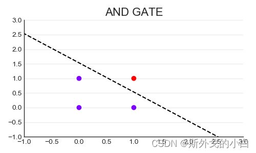
从上图可以看出y=0.15x1+0.15x2-0.23是该样本的完美分割线,说明设置的权重和截距绘制出的直线可以将与门数据的两类点完美分开,就是一条决策边界。
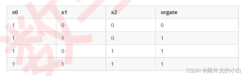
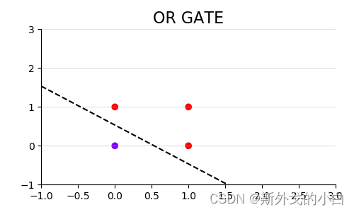
现在,让我们使用阶跃函数作为线性结果之后的函数,在其他典型数据上试试看使用决策边界进行分类的方式。比如下面的“或门”(OR GATE),特征一或特征二为1的时候标签就为1的数据。
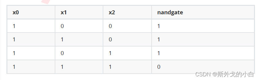
“非与门”(NAND GATE),特征一和特征二都是1的时候标签为0,其他时候标签则为1的数据
或门一阶跃函数为输出的函数值和图像
#定义数据
x = torch.tensor([[1, 0, 0], [1, 1, 0], [1, 0, 1], [1, 1, 1]], dtype=torch.float32)

#定义或门的标签
orgate = torch.tensor([0, 1, 1, 1],dtype=torch.float32)

#或门的函数(基于阶跃函数)
def OR(X):
    w = torch.tensor([-0.08, 0.15, 0.15], dtype=torch.float32)
    zhat = torch.mv(X, w)
    yhat = torch.tensor([torch.ceil(x) for x in zhat], dtype=torch.float32)
    return zhat, yhat

zhat, yhat = OR(X)
print(zhat, yhat)
#tensor([-0.0800,  0.0700,  0.0700,  0.2200]) tensor([-0., 1., 1., 1.])

#绘制直线划分散点的图像
x = np.arange(-1,3,0.5)
plt.figure(figsize=(5,3))
plt.title("OR GATE",fontsize=16)
plt.scatter(X[:,1],X[:,2],c=orgate,cmap="rainbow")
plt.plot(x,(0.08-0.15*x)/0.15,color="k",linestyle="--")
plt.xlim(-1,3)
plt.ylim(-1,3)
plt.grid(alpha=.4,axis="y")
plt.gca().spines["top"].set_alpha(.0)
plt.gca().spines["right"].set_alpha(.0)
plt.show()
非与门以阶跃函数为输出的函数和图像
X = torch.tensor([[1, 0, 0], [1, 1, 0], [1, 0, 1], [1, 1, 1]], dtype=torch.float32)
nandgate = torch.tensor([1, 1, 1, 0], dtype=torch.float32)

def NANDGATE(X):
    w = torch.tensor([0.23, -0.15, -0.15], dtype=torch.float32)
    zhat = torch.mv(X, w)
    yhat = torch.tensor([torch.ceil(i) for i in zhat], dtype=torch.float32)
    return zhat, yhat

zhat, yhat = NANDGATE(X)
print(zhat, yhat)
#tensor([ 0.2300,  0.0800,  0.0800, -0.0700]) tensor([1., 1., 1., -0.])

x = np.arange(-1.3, 5)
plt.figure(figsize=(5, 3))
plt.scatter(X[:, 1], X[:, 2], c=nandgate, cmap="rainbow")
plt.plot(x ,(0.23-0.15*x)/0.15,color="k",linestyle="--")
plt.xlim(-1,3)
plt.ylim(-1,3)
plt.grid(alpha=.4, axis="y")
plt.gca().spines["top"].set_alpha(.0)
plt.gca().spines["right"].set_alpha(.0)
plt.show()
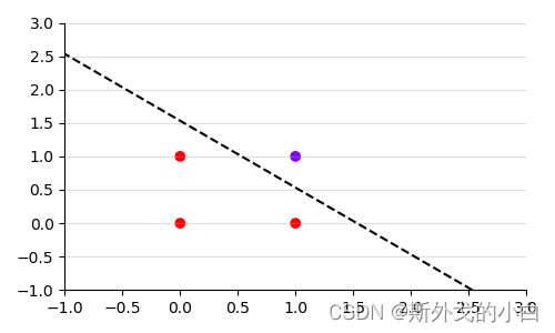
可以看到,或门和非与门的情况都可以被很简单地解决。现在,来看看下面这一组数据:
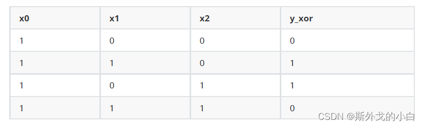 和之前的数据相比,这组数据的特征没有变化,不过标签变成了[0,1,1,0]。这是一组被称为“异或门”(XOR GATE)的数=据,可以看出,当两个特征的取值一致时,标签为0,反之标签则为1。我们同样把这组数据可视化看看:
xorgate = torch.tensor([0, 1, 1, 0], dtype=torch.float32)
plt.figure(figsize=(5, 3))
plt.title("XOR GATE", fontsize=16)
plt.scatter(X[:, 1], X[:, 2], c=xorgate, cmap="rainbow")
plt.xlim(-1, 3)
plt.ylim(-1, 3)
plt.grid(alpha=.4, axis="y")
plt.gca().spines["top"].set_alpha(.0)
plt.gca().spines["right"].set_alpha(.0)
plt.show()
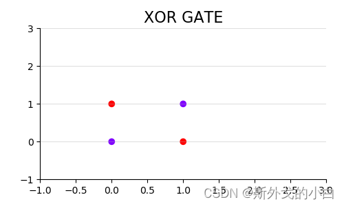
异或门的分割线不能以单纯的一条直线作为决策边界
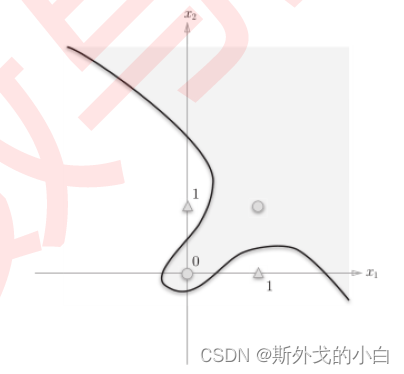
这时我们就要见识一下多层神经网络的厉害之处。当我们将或门和非与门的输出以及列向量进行拼接之后,得到输入与门的适用形状后,通过与门激活得到了异或门的输出。单层的神经网络得不到非线性的决策边界,但是多层神经网络可以,这就是多层神经网络的牛逼之处!
import torch
import numpy as np
from matplotlib import pyplot as plt
import seaborn as sns


X = torch.tensor([[1, 0, 0], [1, 1, 0], [1, 0, 1], [1, 1, 1]], dtype=torch.float32)

#与门
def AND(X):
    w = torch.tensor([-0.2, 0.15, 0.15], dtype=torch.float32)
    zhat = torch.mv(X, w)
    andhat = torch.tensor([torch.ceil(x) for x in zhat], dtype=torch.float32)
    return andhat

#或门
def OR(X):
    w = torch.tensor([-0.08, 0.15, 0.15], dtype=torch.float32)
    zhat = torch.mv(X, w)
    yhat = torch.tensor([torch.ceil(x) for x in zhat], dtype=torch.float32)
    return yhat

def NAND(X):
    w = torch.tensor([0.23, -0.15, -0.15], dtype=torch.float32)
    zhat = torch.mv(X, w)
    yhat = torch.tensor([torch.ceil(x) for x in zhat], dtype=torch.float32)
    return yhat

def XOR(X):
    input_1 = X
    sigma_nand = NAND(input_1)
    sigma_or = OR(input_1)
    x0 = torch.tensor([1, 1, 1, 1])
    #之所以定义x0,是因为我们将要输入到与门,AND(X)一定的w形状是(1, 3),点乘的时候,mv会自动给w转置。所以我们输入的形状必须是(n, 3),由于每个门输出的是一列标签,是(1,4)的形状,所以我们只能将其转置后按列进行拼接
    input_2 = torch.cat((x0.view(4, 1), sigma_nand.view(4, 1), sigma_or.view(4, 1)), dim=1)
    y_and = AND(input_2)
    return y_and

XOR(X)
print(XOR(X))
#tensor([-0., 1., 1., -0.])
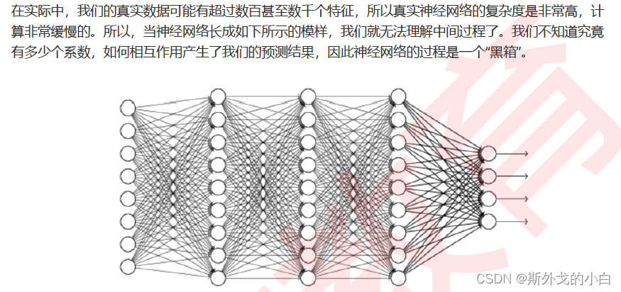
二、黑箱:深层神经网络的不可解释性
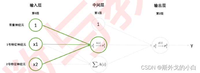
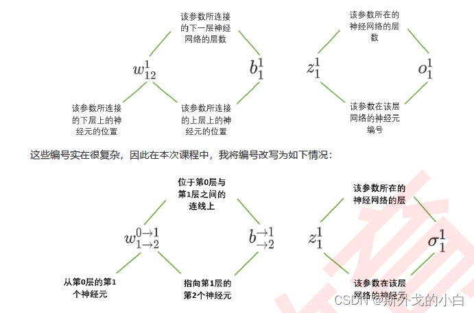

三、探索多层神经网络
代码同上 或异门
四、激活函数
关于激活函数,有以下注意点:
1、虽然都是激活函数,但是隐藏层和输出层上的激活函数作用是完全不一样的。输出层的激活函数是为了让神经网络能够输出不同类型的标签而存在的:softmax激活函数多用于多分类问题中,sigmoid激活函数多用于二分类问题中,阶跃激活函数可以直接用于回归问题中。也就是说,激活函数仅仅与输出结果的表现形式有关,与网络的效果无关。也正因如此,隐藏层的激活函数可以使用阶跃函数。但是隐藏层的激活函数就不同了,隐藏层的激活函数的选择会影响神经网络的效果。
2、在同一个神经网络中,隐藏层的激活函数和输出层的激活函数可以不同。而且在实际运用中,的确是不同的,每一层的激活函数都可以不同,但是同一层上的激活函数一定的一致的。
五、从0实现深度神经网络的正向传播
假设我们现在有500条数据,20个特征,标签为3类,现在需要实现一个三层的神经网络,这个神经网络的架构如下:第一层有13个神经元,第二层有8个神经元,第三层是输出层,其中,第一层的激活函数是relu,第二层的激活函数是sigmoid,如何实现?
#定义数据
torch.random.manual_seed(420)
X = torch.rand((500, 20), dtype=torch.float32)
y = torch.randint(low=0, high=3, size=(500, 1), dtype=torch.float32)

class Model(nn.Module):
    def __init__(self, input_features, out_features):
        super(Model, self).__init__() #super函数是为了将父类的所有函数和属性都继承过来
        #如果没有super函数,就只能继承父类的函数,继承不了父类的属性
        self.Linear1 = torch.nn.Linear(input_features, 13, bias=True)
        self.Linear2 = torch.nn.Linear(13, 8, bias=True)
        self.Output = torch.nn.Linear(8, out_features, bias=True)
    #先定义神经网络的各个线性层,然后定义向前传播

    def forward(self, x):
        z1 = self.Linear1(x)
        sigma1 = torch.relu(z1)
        z2 = self.Linear2(sigma1)
        sigma2 =torch.sigmoid(z2)
        z3 = self.Output(sigma2)
        sigma3 = torch.softmax(z3, dim=1) #对列进行分类,每一个数值都有一个类。
        return sigma3

input_features = X.shape[1]
out_features = len(y.unique()) #分类的书目

#实例化神经网络
torch.random.manual_seed(420)
net = Model(input_features=input_features, out_features=out_features)

print(net(X)) #这两个结果等同是因为类下面只有一个net函数,除了init以外,所以执行类和执行函数的结果一致
print(net.forward(X))
print(net.forward(X).shape)
#torch.Size([500, 3])

#查看标签
sima = net.forward(X)
print(sima.max(axis=1)) #取出标签中每一行上最大值就成为我们的预测类别


print(net.Linear1.weight)
print(net.Linear1.weight.shape)
#torch.Size([13, 20]) 权重矩阵的形状和神经元的形状正好反过来了
print(net.Linear2.weight.shape)
#torch.Size([8, 13])
测试super中重要性
class FooParent(object):
	def __init__(self):
	self.parent = 'PARENT!!'
	print ('Running __init, I am parent')

	def bar(self,message):
	self.bar = "This is bar"
	print ("%s from Parent" % message)

FooParent() #父类实例化的瞬间,运行自己的__init__
FooParent().parent #父类运行自己的__init__中定义的属性
#建立一个子类,并通过类名调用让子类继承父类的方法与属性
class FooChild(FooParent):
	def __init__(self):
	print ('Running __init, I am child')
	#查看子类是否继承了方法
	FooChild().bar("HAHAHA")

FooChild().parent #子类没有继承到父类的__init__中定义的属性
#为了让子类能够继承到父类的__init__函数中的内容,我们使用super函数
#新建一个子类,并使用super函数
class FooChild(FooParent):
def __init__(self):
super(FooChild,self).__init__()
print ('Child')
print ("I am running the __init__")
#再次调用parent属性
FooChild() #执行自己的init功能的同时,也执行了父类的init函数定义的功能
FooChild().parent
结果就是,如果不写super这个内容,子类只能继承父类的函数,不能继承其属性。


 被折叠的 条评论
为什么被折叠?
被折叠的 条评论
为什么被折叠?
 到【灌水乐园】发言


