2.1 探索性数据分析

2.1 探索性数据分析

2.1 数据预处理之探索性数据分析

本节课的ppt：eda slides

1.导入相关包

00:47

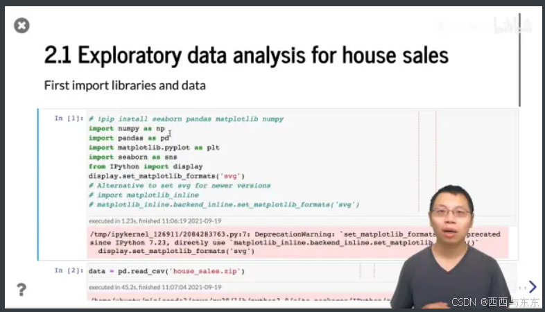numpy：python中做数据分析常用的包；

pandas：也是用于数据分析，擅长处理表，数据没那么大要放入内存中，这将是首选；

matplotlib.pyplot：源自matlab的画图工具；

seaborn：基于matplotlib，提供更多的画法

剩下两行用于将图片设成svg文件（画起来分辨率相对高一点）

==================

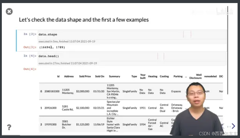
2.读取数据

03:07

csv文件存下来相对比较大，可以先压缩成一个zip或一个tar，主流的读取文件都可以从压缩文件中读取。建议存成压缩文件，在传输存储都会比较好，甚至还会比直接读取还要好（这个方法可用于文本）

看看读了多少东西出来

05:09

data.head() 把前面几行信息打出来

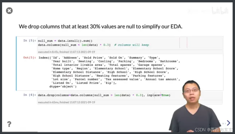
将列中30%缺失的列删去，以此来简化数据

06:59

In[6] 中的 inplace的作用是，直接将要去掉的列给改写掉（直接对数进行修改），可以省些内存，但是这个只能跑一次

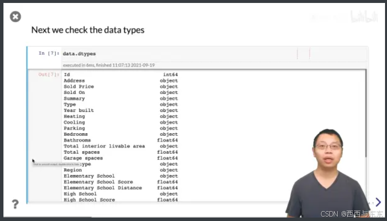
看看存的那些列的数据类型是否正确

09:21

处理错误的数据类型

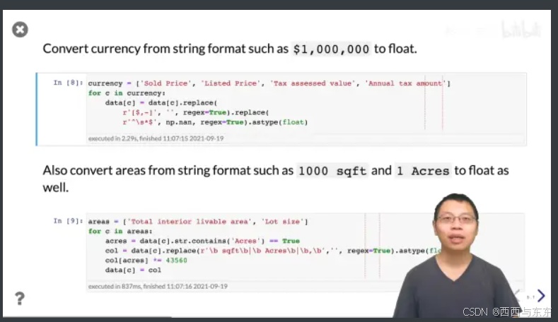
最后用data.describe()看看处理完的数据的特征

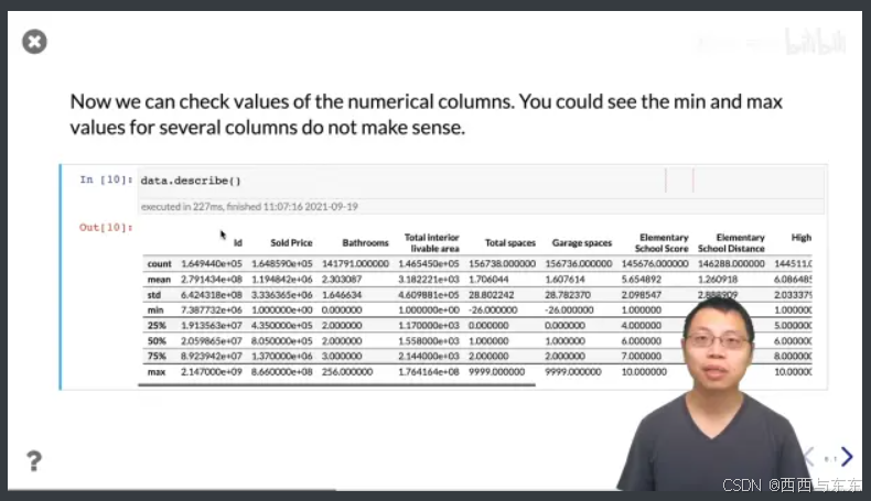可以通过这里初步判断是否有噪音

==================

做简单的处理

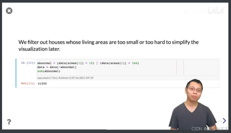
16:34

把不正常的数据去除

看看卖的价格的分布

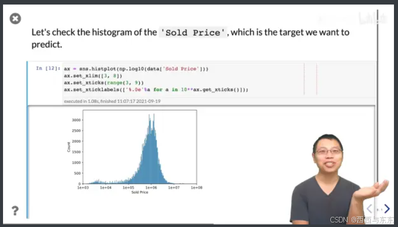
17:53

在这里用log10可以让分布均匀点

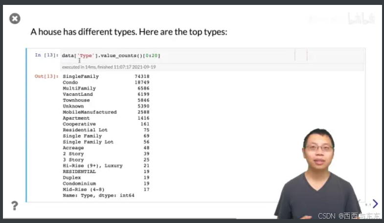
看看房子的种类

20:09

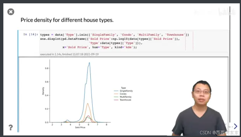
看看不同类别的房子是什么价格

21:39

看看一平米可以卖多少钱

23:57

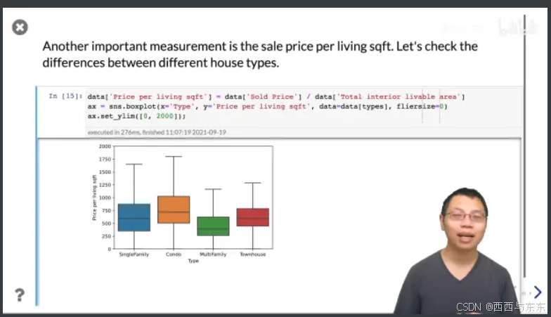不同颜色是不同类别，那条横线表示的是均值，boxplot可以比较直观的看到不同分布之间的对比

看看每个邮政编码的房价

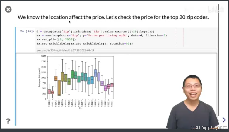
27:27

看看每个特征之间的关系（协方差）

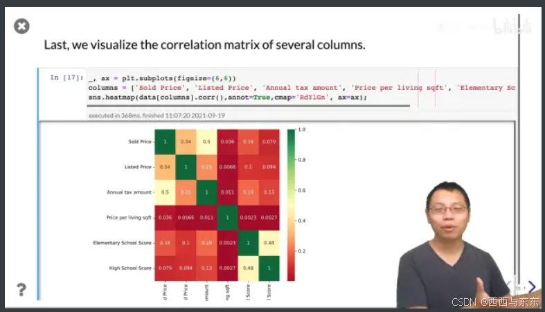
28:34

可以直观的看出，谁跟我要预测的东西关联度最高

==================

总结

32:10

# 前言

课程地址：2.1 探索性数据分析【斯坦福21秋季：实用机器学习中文版】

数据集地址：Assignments — Practical Machine Learning

原版代码：eda slides

数据集不同导致的各种问题

1.最后输出图片时只能输出(4*4)的图片

2.输出地域箱形图时失真

个人解决方式：

```python

data['Id']=data['Id'].astype(int)

data['Elementary School Score']=data['Elementary School Score'].astype(float)

data['Total spaces']=data['Total spaces'].astype(float)

data['Bathrooms']=data['Bathrooms'].astype(float)

data['Elementary School Distance']=data['Elementary School Distance'].astype(float)

data['Bathrooms']=data['Bathrooms'].astype(float)

data['Garage spaces']=data['Garage spaces'].astype(float)

data['Zip']=data['Zip'].astype(int)

```

复现代码：

#!/usr/bin/env python
 # coding: utf-8
 ​
 # In[1]:
 ​
 ​
 # !pip install seaborn pandas matplotlib numpy
 import numpy as np
 import pandas as pd
 import matplotlib.pyplot as plt
 import seaborn as sns
 from IPython import display
 display.set_matplotlib_formats('svg')
 # Alternative to set svg for newer versions
 # import matplotlib_inline
 # matplotlib_inline.backend_inline.set_matplotlib_formats('svg')
 ​
 ​
 # In[2]:
 ​
 ​
 data = pd.read_feather('house_sales.ftr')
 ​
 ​
 # In[3]:
 ​
 ​
 data.shape
 ​
 ​
 # In[4]:
 ​
 ​
 data.head(10)
 ​
 ​
 # In[5]:
 ​
 ​
 null_sum = data.isnull().sum()
 data.columns[null_sum < len(data)*0.3]
 ​
 ​
 # In[6]:
 ​
 ​
 data.drop(columns = data.columns[null_sum > len(data) * 0.3],inplace=True)
 ​
 ​
 # In[7]:
 ​
 ​
 data['Id']=data['Id'].astype(int)
 data['Elementary School Score']=data['Elementary School Score'].astype(float)
 data['Total spaces']=data['Total spaces'].astype(float)
 data['Bathrooms']=data['Bathrooms'].astype(float)
 data['Elementary School Distance']=data['Elementary School Distance'].astype(float)
 data['Bathrooms']=data['Bathrooms'].astype(float)
 data['Garage spaces']=data['Garage spaces'].astype(float)
 data['Zip']=data['Zip'].astype(int)
 ​
 ​
 # In[8]:
 ​
 ​
 data.dtypes
 ​
 ​
 # In[9]:
 ​
 ​
 currency = ['Sold Price','Listed Price','Tax assessed value','Annual tax amount']
 for c in currency:
     data[c] = data[c].replace(
     r'[$,-]','',regex=True).replace(
     r'^\s*$',np.nan,regex=True).astype(float)
 ​
 ​
 # In[10]:
 ​
 ​
 areas=['Total interior livable area','Lot size']
 for c in areas:
     acres = data[c].str.contains('Acres') == True
     col = data[c].replace(r'\b sqft\b|\b Acres\b|\b,\b','',regex=True).astype(float)
     col[acres]*=43560
     data[c]=col
 ​
 ​
 # In[11]:
 ​
 ​
 data.describe()
 ​
 ​
 # In[12]:
 ​
 ​
 abnormal = (data[areas[1]] < 10) | (data[areas[1]] > 1e4)
 data = data[~abnormal]
 sum(abnormal)
 ​
 ​
 # In[13]:
 ​
 ​
 ax = sns.histplot(np.log10(data['Sold Price']))
 ax.set_xlim([3, 8])
 ax.set_xticks(range(3, 9))
 ax.set_xticklabels(['%.0e'%a for a in 10**ax.get_xticks()]);
 ​
 ​
 # In[14]:
 ​
 ​
 data['Type'].value_counts()[0:20]
 ​
 ​
 # In[15]:
 ​
 ​
 types = data['Type'].isin(['SingleFamily', 'Condo', 'MultiFamily', 'Townhouse'])
 sns.displot(pd.DataFrame({'Sold Price':np.log10(data[types]['Sold Price']),
                           'Type':data[types]['Type']}),
             x='Sold Price', hue='Type', kind='kde');
 ​
 ​
 # In[16]:
 ​
 ​
 #箱式图
 data['Price per living sqft'] = data['Sold Price'] / data['Total interior livable area']
 ax = sns.boxplot(x='Type', y='Price per living sqft', data=data[types], fliersize=0)
 ax.set_ylim([0, 2000]);
 #中间横线是中位数
 #上面的横线是最大值
 #方框上边界为3/4的值
 ​
 ​
 # In[17]:
 ​
 ​
 d = data[data['Zip'].isin(data['Zip'].value_counts()[:20].keys())]
 ax = sns.boxplot(x='Zip', y='Price per living sqft', data=d, fliersize=0)
 ax.set_ylim([0, 2000])
 ax.set_xticklabels(ax.get_xticklabels(), rotation=90);
 ​
 ​
 # In[18]:
 ​
 ​
 data.dtypes
 ​
 ​
 # In[19]:
 ​
 ​
 _, ax = plt.subplots(figsize=(6,6))
 columns = ['Sold Price', 'Listed Price', 'Annual tax amount', 'Price per living sqft', 'Elementary School Score', 'High School Score']
 sns.heatmap(data[columns].corr(),annot=True,cmap='RdYlGn', ax=ax);
 ​
 ​
 # In[ ]: